Download
1 / 23
240 likes | 863 Views
Sensitivity analysis. It refers to the study of coefficient changes of decision variables that would not affect to the optimal solution we obtained What does it mean? Tutorial. (to p2). (to p19). Consider the following LP problem:. Solution: z= 2,240, x1=4, x2=8, and s3=48.

E N D
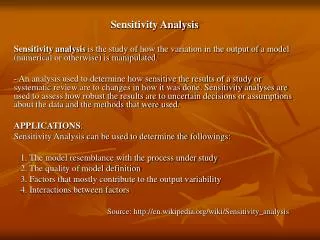
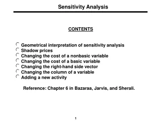
Sensitivity analysis • It refers to the study of coefficient changes of decision variables that would not affect to the optimal solution we obtained • What does it mean? • Tutorial (to p2) (to p19)
Consider the following LP problem: Solution: z= 2,240, x1=4, x2=8, and s3=48 Question: what range of Cj values can be changed and yet the optimal solution remains unchanged? (to p3) Two groups of coefficients could be studied …….
Sensitivity Analysis Two groups of coefficients could be changed: • The objective function cost cj • The constraint quantities bi • Semantic view • Procedural steps for sensitivity analysis (to p4) (to p5)
Semantic view bi Cj (to p3)
Procedural Steps • Change of objective function cost cj • Change of constraint quantity bi (to p6) (to p12) (to p1)
Change of objective function cost cj Consider the following optimal tableau: Here, we are to study what value can Cj be changed and yet the above optimal solution remains unchanged. Let consider C1, and let ▲ be the change of C1, then C1 = 160 + ▲, replacing this to the above tableau, we have … (to p7)
Cj analysis Again, we follow the normal procedure and compute the solution until all values of cj-zj≤ 0, then we have Solve these two equations …. (to p8)
c1 (to p9) We can repeat these steps for c2 too
c2 (to p10) Solve these two inequalities, we have …
c2 (to p11) Important note!
Important note! For c1 and c2 Thus, we can only consider them ONE at a time only! (to p5)
Change of constraint quantity bi Consider the following: Here, we can analyze b1, b2, and b3,and its corresponding slack variables are s1, s2, and s2 (why?) Then, we analyze the changes of b1, b2, and b3 independently since each has a different slack variables How? …. (to p13)
Analysis of bi • Three bi can be analyzed: • b1 • b2 • b3 (to p14) (to p16) (to p18) (to p5)
b1 Here, we multiple s1 to the total quantity, and solve ▲ Now, all bi ≥ 0, then (to p15) Continue..
b1 (to p13)
b2 (to p17) Continue …
b3 In a similar vein, we get .. Please try q3 at home! (to p13)
Tutorial • See the following slides for these full questions: • 48 b-f, 49a-e, 50 b-d • Also run and compare their computer outputs!