Download
1 / 45
450 likes | 698 Views
Multivariate Statistical Data Analysis with Its Applications. Hua-Kai Chiou Ph.D., Assistant Professor Department of Statistics, NDMC hkchiou@rs590.ndmc.edu.tw. September, 2005. Agenda. Introduction Examining Your Data Sampling & Estimation Hypothesis & Testing

E N D
Multivariate Statistical Data Analysis with Its Applications Hua-Kai Chiou Ph.D., Assistant Professor Department of Statistics, NDMC hkchiou@rs590.ndmc.edu.tw September, 2005
Agenda • Introduction • Examining Your Data • Sampling & Estimation • Hypothesis & Testing • Multiple Regression Analysis • Logistic Regression • Multivariate Analysis of Variance • Principal Components Analysis
Factor Analysis • Cluster Analysis • Discriminant Analysis • Multidimensional Scaling • Canonical Correlation Analysis • Conjoint Analysis • Structural Equation Modeling
1 Introduction
Some Basic Concept of MVA • What is Multivariate Analysis (MVA)? • Impact of the Computer Revolution • Multivariate Analysis Defined • Measurement Scales • Type of Multivariate Techniques
Dependence technique – the objective is prediction of the dependent variable(s) by the independent variable(s), e.g., regression analysis. • Dependent variable – presumed effect of, or response to, a change in the independent variable(s). • Dummy variable – nometrically measured variable transformed into a metric variable by assigning 1 or 0 to a subject, depending on whether it possesses a particular characteristic. • Effect size – estimate of the degree to which the phenomenon being studied (e.g., correlation or difference in means) exists in population.
Indicator – single variable used in conjunction with one or more other variables to form a composite measure. • Interdependence technique – classification of statistical techniques in which the variables are not divided into dependent and independent sets (e.g., factor analysis). • Metric data – also called quantitative data, interval data, or ratio data, these measurements identify or describe subjects (or objects) not only on the possession of an attribute but also by the amount or degree to which the subject may be characterized by attribute. For example, a person’s age and weight are metric data.
Multicollinearity – extent to which a variable can be explained by the other variables in the analysis. As multicollinearity increases, it complicates the interpretation of the variate as it is more difficult to ascertain the effect of any single variable, owing to their interrelationships. • Nonmetric data – also called qualitative data. • Power – probability of correctly rejecting the null hypothesis when it is false, that is, correctly finding a hypothesized relationship when it exists. Determined as a function of (1)the statistical significance level (α) set by the researcher for a Type I error, (2) the sample size used in the analysis, and (3) the effect size being examined.
Practical significance – means of assessing multivariate analysis results based on their substantive findings rather than their statistical significance. Whereas statistical significance determines whether the result is attributable to chance,practical significance assesses whether the result is useful. • Reliability – extent to which a variable or set of variables is consistent in what it is intended to measure. Reliability relates to the consistency of the measure(s). • Validity – extent to which a measure or set of measures correctly represents the concept of study. Validity is concerned with how well the concept is defined by the measure(s).
Type I error – probability of incorrectly rejecting the null hypothesis. • Type II error - probability of incorrectly failing to reject the null hypothesis, it meaning the chance of not finding a correlation or mean difference when it does exist. • Variate – linear combination of variables formed in the multivariate technique by deriving empirical weights applied to a set of variables specified by the researcher.
The Relationship between Multivariate Dependence Methods Analysis of Variance (ANOVA) (metric) (nometric) Multivariate Analysis of Variance (MANOVA) (metric) (nometric) Canonical Correlation (metric, nometric) (metric, nometric)
Discriminant Analysis (nometric) (metric) Multiple Regression Analysis (metric) (metric, nometric) Conjoint Analysis (metric, nometric) (nometric)
Structural Equation Modeling (metric) (metric, nometric)
What type of relationship is being examined? Dependence Interdependence How many variables are being predicted? Is the structure of relationships among: Multiple relationships of dependent and independent variables Several dependent variables in single relationship One dependent variables in single relationship Variable Cases/Respondent Object Factor analysis Cluster analysis How are the attributes measured? Structural Equation Modeling What is the measurement scale of the dependent variable? What is the measurement scale of the dependent variable? Metric Nometric Nometric Metric Nometric Metric Nometric Multidimensional scaling Correspondence analysis What is the measurement scale of the dependent variable? Canonical correlation analysis with dummy variables Multiple discriminant analysis Linear probability models Multiple regression Conjoint analysis Metric Nometric Canonical correlation analysis Multivariate analysis of variance (MANOVA)
A Structured Approach to Multivariate Model Building Stage 1: Define the research problem, objectives, and multivariate technique to be used Stage 2: Develop the analysis plan Stage 3: Evaluate the assumptions underlying the multivariate technique Stage 4: Estimate the multivariate model and assess overall model fit Stage 5: Interpret the variate(s) Stage 6: Validate the multivariate model
2 Examining Your Data
HATCO Case • Primary Database • This example investigates a business-to-business case from existing customers of HATCO. • The primary database consists 100 observations on 14 separate variables. • Three types of information were collected: • The perceptions of HATCO, 7 attributes (X1 – X7); • The actual purchase outcomes, 2 specific measures (X9,X10); • The characteristics of the purchasing companies, 5 characteristics (X8, X11-X14).
Table 2.1 Description of Database Variables (Hair et al., 1998)
Fig 2.1 Scatter Plot Matrix of Metric Variables (Hair et al., 1998)
Fig 2.2 Examples of Multivariate Graphical Displays (Hair et al., 1998)
Missing Data • A missing data process is any systematic event external to the respondent (e.g. data entry errors or data collection problems) or action on the part of the respondent (such as refusal to answer) that leads to missing values. • The impact of missing data is detrimental not only through its potential “hidden” biases of the results but also in its practical impact on the sample size available for analysis.
Understanding the missing data • Ignorable missing data • Remediable missing data • Examining the pattern of missing data
Table 2.2 Summary Statistics of Pretest Data (Hair et al., 1998)
Table 2.3 Assessing the Randomness of Missing Data through Group Comparisons of Observations with Missing versus Valid Data (Hair et al., 1998)
Table 2.4 Assessing the Randomness of Missing Data through Dichotomized Variable Correlations and the Multivariate Test for Missing Completely at Random (MCAR) (Hair et al., 1998)
Table 2.5 Comparison of Correlations Obtained with All-Available (Pairwise), Complete Case (Listwise), and Mean Substitution Approaches (Hair et al., 1998)
Table 2.6 Results of the Regression and EM Imputation Methods (Hair et al., 1998)
Outliers • Four classes of outliers: • Procedural error • Extraordinary event can be explained • Extraordinary observations has no explanation • Observations fall within the ordinary range of values on each of the variables but are unique in their combination of values across the variables. • Detecting outliers • Univariate detection • Bivariate detection • Multivariate detection
Outliers detection • Univariate detection threshold: • For small samples, within ±2.5 standardized variable values • For larger samples, within ±3 or ± 4 standardized variable values • Bivariate detection threshold: • Varying between 50 and 90 percent of the ellipse representing normal distribution. • Multivariate detection: • The Mahalanobis distance D2
Table 2.7 Identification of Univariate and Bivariate Outliers (Hair et al., 1998)
Fig 2.3 Graphical Identification of Bivariate Outliers (Hair et al., 1998)
Table 2.8 Identification of Multivariate Outliers (Hair et al., 1998)
Testing the Assumptions of Multivariate Analysis • Graphical analyses of normality • Kurtosis refers to the peakedness or flatness of the distribution compared with the normal distribution. • Skewness indicates the arc, either above or below the diagonal. • Statistical tests of normality
Fig 2.4 Normal Probability Plots and Corresponding Univariate Distribution (Hair et al., 1998)
Homoscedasticity vs. Heteroscedasticity • Homoscedasticity is an assumption related primarily to dependence relationships between variables. • Although the dependent variables must be metric, this concept of an equal spread of variance across independent variables can be applied either metric or nonmetric.
Fig 2.5 Scatter Plots of Homoscedastic and Heteroscedastic Relationships (Hair et al., 1998)
Fig 2.6 Normal Probability Plots of Metric Variables (Hair et al., 1998)
Table 2.9 Distributional Characteristics, Testing for Normality, and Possible Remedies (Hair et al., 1998)
Fig 2.7 Transformation of X2 (Price Level) to Achieve Normality (Hair et al., 1998)
3 Sampling Distribution
Understandingsampling distributions • A histogram is constructed from a frequency table. The intervals are shown on the X-axis and the number of scores in each interval is represented by the height of a rectangle located above the interval.
A bar graph is much like a histogram, differring in that the columns are separated from each other by a small distance. Bar graphs are commonly used for qualitative variables.
What is a normal distribution? • Normal distributions are a family of distributions that have the same general shape. They are symmetric with scores more concentrated in the middle than in the tails. Normal distributions are sometimes described as bell shaped. The height of a normal distribution can be specified mathematically in terms of two parameters: the mean (m) and the standard deviation (s).