Download
1 / 67
680 likes | 825 Views
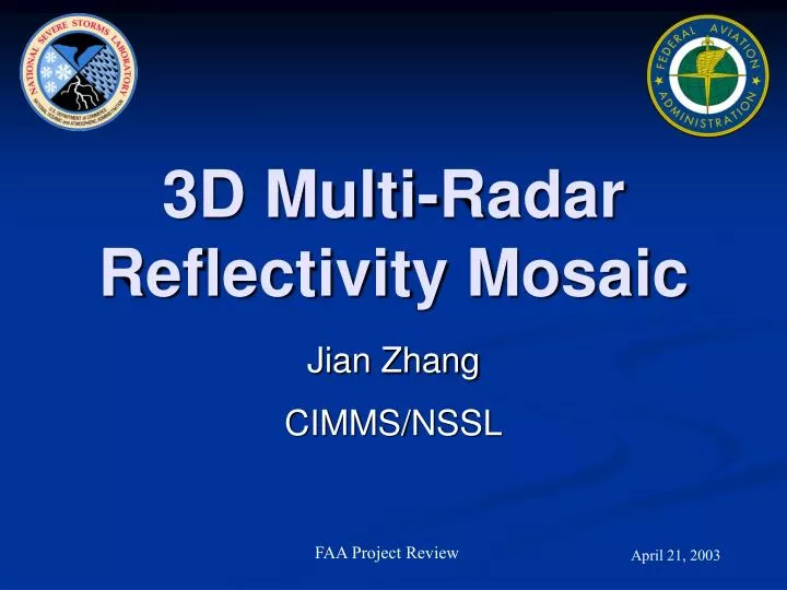
3D Multi-Radar Reflectivity Mosaic. Jian Zhang CIMMS/NSSL. April 21, 2003. FAA Project Review. OUTLINE. Motivation Challenges WSR-88D data characteristics Demo of various gridding schemes Demo of various mosaicking schemes Summary. Why Mosaic. Single radar has limited coverage

E N D
3D Multi-Radar Reflectivity Mosaic Jian Zhang CIMMS/NSSL April 21, 2003 FAA Project Review
OUTLINE • Motivation • Challenges • WSR-88D data characteristics • Demo of various gridding schemes • Demo of various mosaicking schemes • Summary
Why Mosaic • Single radar has limited coverage • Weather systems span over multiple radar umbrellas • FAA ARTCCs span multiple radar umbrellas (multiple states) • Multi-sensor storm algorithms require radar data on a common grid as other data (e.g., satellite, lightning, etc)
Why 3D Mosaic • 2D radar mosaic products have been very useful and efficient in many operational weather decision making processes • Adding high resolution vertical structure data can: • Provide more info about aviation hazardous weather • Help develop more and better aviation weather products • More efficient air traffic routing and improved aviation safety • Other: • Help improve storm growth and decay analysis • More accurate QPE • Help improve convective scale numerical weather prediction
Challenges for 3D Multi-radar Mosaic • Extremely non-uniform data resolution • Different weather types/regimes • Non-weather echo contamination/quality control • Calibration differences • Synchronization among radars • Computational efficiency in real-time application
Choose a Filter for Gridding: Uniform or Adaptive? • Uniform: (Trapp and Doswell, 2000, JTECH,17) • Scale uniformity • Adaptive: (Askelson et al. 2000, MWR, 128) • Minimize RMS error • Retain high-resolution info in radar data • Depends on radar data characteristics and applications
WSR-88D Radar Beam Propagation • Effective earth’s radius model (Doviak and Zrnic,1984): h: height above the earth surface r: slant range s: distance along the earth surface
Radar Beam Propagation • Assumptions: • Spherically stratified atmosphere • Refractive index of air, n(h), linearly changes with height, h; • |n-1|<< 1 • Predicts beam height with sufficient accuracy for exponential reference atmosphere • Severe departures at lower atmosphere (“AP”): • Temperature inversions • Large moisture gradients
WSR-88D Data Resolution • Spatial resolution of radar data: • In spherical coordinates: • ~1x 1km x 1 at lower tilts (azimuth:range:elevation) • higher tilts are as far as 5 apart • Power density distribution not point data • “Effective” spatial resolution of radar data: • Physical distance between centers of adjacent radar bins in space
WSR-88D Azimuthal Resolution (VCP11 and VCP21) Azimuthal resolution is worse than 1km beyond 60 km range
Choose a Filter: Uniform or Adaptive? • Our choice: adaptive • Largely different spatial resolution • An adaptive filter is needed for gridding radar data in order to retain high resolution info in radar data • Data sampling resolution are worse than 1km in most places: • Grid resolution of 1km is sufficient
Demo of Gridding Schemes • Gridding Schemes • “Resolution volume mapping” • Nearest neighbor • Vertical interpolation (adaptive) • Vertical interpolation plus gap-filling • Cases: • convective, 6/25/02, 2036Z, KIWX • stratiform, 2/15/98, 0859Z, KIWA
Gridding Scheme I: Resolution Volume Mapping • Assuming each radar bin (resolution volume) size =1x 1km x 1 • Resample on Cartesian grid • Usually 1km x 1km x 500m • For any given grid cell, if the center of the grid cell is inside a radar bin volume, then the grid cell will take the value of the radar bin. • Like nearest neighbor, but within the beam width. Gaps may exists.
Gridding Scheme II:Nearest Neighbor • For each grid cell: • If the center is above (below) the highest (lowest) elevation angle, but within half of a beam width, then it will take the value of the nearest bin value on the highest (lowest) tilt. • If the center is in between the lowest and highest elevation angles, then it will take the value of the nearest radar bin. • No gaps between the lowest and highest tilts
Convective Case1: RHI, 263° Resolution Volume Mapping Nearest Neighbor
Convective Case1: RHI, 173° Resolution Volume Mapping Nearest Neighbor
Convective Case1: CAPPI, 5km Resolution Volume Mapping Nearest Neighbor
Convective Case1: CAPPI, 12km Resolution Volume Mapping Nearest Neighbor
Stratiform Case 2: RHI, 0° Resolution Volume Mapping Nearest Neighbor
Stratiform Case2: CAPPI, 2.3km Resolution Volume Mapping Nearest Neighbor
Stratiform Case2: CAPPI, 5km Resolution Volume Mapping Nearest Neighbor
Gridding Scheme I Summary:Resolution Volume Mapping • Shows raw data distribution • Gaps between high tilts • Ring-shaped discontinuities, especially for stratiform echoes. Caused by the coarse vertical resolution.
Gridding Scheme II Summary:Nearest Neighbor • No smoothing • Gaps are filled • Ring-shaped discontinuities
Gridding Scheme III:Vertical Adaptive Barnes • For each grid cell: • If the center is above (below) the highest (lowest) elevation angle, same as the nearest neighbor. • If the center is in between the lowest and highest elevation angles, then it will take the weighted mean of the two nearest radar bin values, one at the tilt above and one at below.
Convective Case1: RHI, 263° Nearest Neighbor Vertical Adaptive Barnes
Convective Case1: RHI, 173° Nearest Neighbor Vertical Adaptive Barnes
Convective Case1: CAPPI, 5km Nearest Neighbor Vertical Adaptive Barnes
Convective Case1: CAPPI, 12km Vertical Adaptive Barnes Nearest Neighbor
Stratiform Case 2: RHI, 0° Nearest Neighbor Vertical Adaptive Barnes
Stratiform Case2: CAPPI, 2.3km Vertical Adaptive Barnes Nearest Neighbor
Stratiform Case2: CAPPI, 5km Nearest Neighbor Vertical Adaptive Barnes
Gridding Scheme III Summary:Vertical Adaptive Barnes • Filled gaps • Alleviated discontinuities • Bright-band rings still exist
Gridding Scheme IV:Adaptive Barnes + Gap Filling • For each grid cell: • If the center is above (below) the highest (lowest) elevation angle, same as the nearest neighbor. • If the center is in between the lowest and highest elevation angles, then it will take the weighted mean of four radar bin values on the tilt above and below, all at the same azimuth. Two of the radar bins are at the same range and two others are at the same height as the grid cell (See Figure next)
Stratiform Case 2: RHI, 0° Vertical Adaptive Barnes Adaptive Barnes + Gap Filling
Stratiform Case2: CAPPI, 2.3km Adaptive Barnes + Gap Filling Vertical Adaptive Barnes
Convective Case1: RHI, 263° Vertical Adaptive Barnes Adaptive Barnes + Gap Filling
Gridding Scheme IV Summary:Adaptive Barnes + Gap Filling • Filled gaps • Eliminated discontinuities • Alleviated bright-band rings • Not suited for upright convective systems, so…. • Solution: • Apply gap filling component only when bright-band is identified (Gourley and Calvert 2003) • Constraints: • h/s > scale_ratio; • range < range_limit;
Mosaic • Data from individual radars have now been gridded (resampled on Cartesian grid) • Now we need to combine or mosaic data from multiple radars
Mosaic Scheme I: Nearest Neighbor • At each grid cell: • If there is only one radar’s grid value, then the value is used • If there are multiple radar values, then the value from the nearest radar is used.
Mosaic Scheme II: Maximum • At each grid cell: • If there is only one radar’s grid value, then the value is used • If there are multiple radar values, the the maximum value among the multiple radars is used.