Ohio’s Rural Streams: Flashy and Getting Flashier D. B. Baker, R. P. Richards, T. T. Loftus, and J. W. Kramer, Water Qua

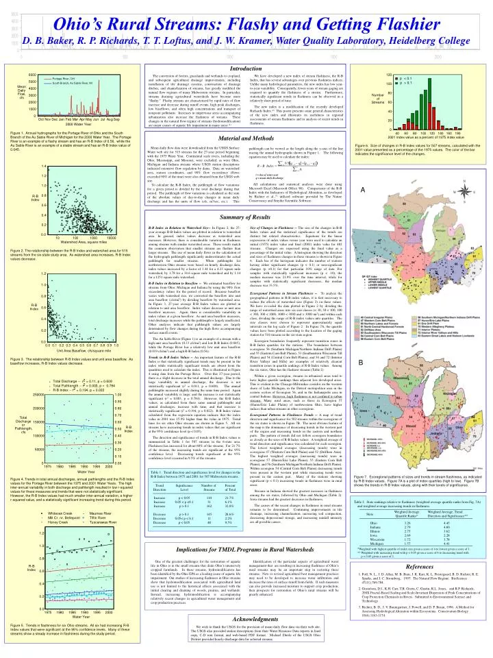
1. Acknowledgments      We wish to thank the USGS for the provision of mean daily flow data via their web site. The USGS also provided station descriptions from their Water Resource Data reports in hard copy, C-D rom format, and web-based PDF format. Michael Eberle of the USGS Ohio District provided hourly discharge data for selected streams. Ohio’s Rural Streams: Flashy and Getting Flashier D. B. Baker, R. P. Richards, T. T. Loftus, and J. W. Kramer, Water Quality Laboratory, Heidelberg College Introduction The conversion of forests, grasslands and wetlands to cropland, and subsequent agricultural drainage improvements, including installation of tile drainage systems, construction of drainage ditches, and channelization of streams, has greatly modified the natural flow regimes of many Midwestern streams. In particular, streams draining agricultural watersheds have become more “flashy.” Flashy streams are characterized by rapid rates of flow increase and decrease during runoff events, high peak discharges, low baseflows, and often high concentrations and transport of nonpoint pollutants. Increases in impervious areas accompanying urbanization also increase the flashiness of streams. These changes in the natural flow regime of streams (hydromodification) are major causes of aquatic life impairment in many areas.(1) We have developed a new index of stream flashiness, the R-B Index, that has several advantages over previous flashiness indices. Unlike many hydrological parameters, the new index has low year-to-year variability. Consequently, fewer years of stream gaging are required to quantify the flashiness of a stream. Furthermore, statistically significant trends in flashiness can be observed in a relatively short period of time. The new index is a modification of the recently developed Richards Index.(2) This poster presents some general characteristics of the new index and illustrates its usefulness in regional assessments of stream flashiness and in analysis of recent trends in flashiness. Figure 1. Annual hydrographs for the Portage River of Ohio and the South Branch of the Au Sable River of Michigan for the 2000 Water Year. The Portage River is an example of a flashy stream and has an R-B Index of 0.56, while the Au Sable River is an example of a stable stream and has an R-B Index value of 0.045. Material and Methods Figure 6. Size of changes in R-B Index values for 507 streams, calculated with the 2001 value presented as a percentage of the 1975 values. The color of the bar indicates the significance level of the changes. Mean daily flow data were downloaded from the USGS Surface Water web site for 515 streams for the 27-year period beginning with the 1975 Water Year. Continental scale rivers, including the Ohio, Mississippi, and Missouri, were excluded, as were Ohio, Michigan and Indiana streams where USGS station descriptions indicated extensive flow regulation by dams. Data on watershed area, station coordinates, and 90% flow exceedency (flows exceeded 90% of the time) were also obtained from the USGS web site. To calculate the R-B Index, the pathlength of flow variations for a given period is divided by the total discharge during that period. The pathlength of flow variations is calculated as the sum of the absolute values of day-to-day changes in mean daily discharge and has the units of flow (cfs, m3/sec, etc.). This pathlength can be viewed as the length along the y-axis of the line tracing the annual hydrographs shown in Figure 1. The following equation may be used to calculate the index: t = day of water year q = mean daily discharge All calculations and statistical analyses were done using Microsoft Excel (Microsoft Office 98). Comparisons of the R-B Index with the Indicators of Hydrological Alteration, as developed by Richter et al.,(3) utilized software provided by The Nature Conservancy and Smythe Scientific Software. A Summary of Results R-B Index in Relation to Watershed Size-- In Figure 2, the 27-year average R-B Index values are plotted in relation to watershed area. In general, index values decrease as watershed area increases. However, there is considerable variation in flashiness among streams with similar watershed areas. These results match the common observation that smaller streams are flashier than larger streams. The use of mean daily flows in the calculation of the hydrograph pathlength significantly underestimates the actual pathlength for smaller streams. When pathlengths for northwestern Ohio streams were based on hourly discharge data, index values increased by a factor of 3.44 for a 4.23 square mile watershed, by 1.78 for a 34.6 square mile watershed and by 1.14 for a 1251 square mile watershed. R-B Index in Relation to Baseflow -- We estimated baseflow for streams from Ohio, Michigan and Indiana by using the 90% flow exceedency values for the period of record. Because baseflow varies with watershed size, we converted the baseflow into unit area baseflow (cfs/mi2) by dividing baseflow by watershed area. In Figure 3, 27-year average R-B Index values are plotted in relation to unit area baseflow. Index values decrease as unit area baseflow increases. Again, there is considerable variability in index values at a given baseflow. As unit area baseflow increases, total discharge increases while the pathlength is largely unaffected. Other analyses indicate that pathlength values are largely determined by flow changes during the high flows accompanying surface runoff events. The Au Sable River (Figure 1) is an example of a stream with a high unit area baseflow (0.33 cfs/mi2) and low R-B Index (0.045), while the Portage River has a relatively low unit area baseflow (0.019 cfs/mi2) and a high R-B Index (0.56). Trends in R-B Index Values --An important feature of the R-B Index is that statistically significant trends may be present in the index while statistically significant trends are absent from the quantities used to calculate the index. This is illustrated in Figure 4 using data from the Portage River. Over this 27-year period, there is a slight decrease in the total annual discharge. Due to the large variability in annual discharge, the decrease is not statistically significant (r2 = 0.011, p = 0.609). The annual pathlengths increased slightly during the same time period. Again the annual variability is large, and the increase is not statistically significant (r2 = 0.003, p = 0.784). However, the R-B Index values, as calculated from these same annual pathlengths and annual discharges, increase with time, and that increase is statistically significant (r2 = 0.194, p = 0.022). R-B Index values calculated from the regression equation indicate that the index value in 2001 was 15.9% higher than the value in 1975. Trend lines for six other Ohio streams are shown in Figure 5. All six streams have increasing trends in index values that are significant at the 95% confidence level (p < 0.05). The direction and significance of trends in R-B Index values is summarized in Table 1 for 507 streams in the 6-state area. Flashiness has increased for about 60% of the streams. For 21.7% of the streams, the increasing trends are significant at the 95% confidence level. Decreasing trends significant at the 95% confidence level occurred in 9.5% of the streams. Size of Changes in Flashiness -- The size of the changes in R-B Index values and the statistical significance of the trends are distinct but related characteristics. Equations for the linear regressions of index values versus year were used to calculate an initial (1975) index value and final (2001) index value for 482 streams. Changes are expressed using the final value as a percentage of the initial value. A histogram showing the direction and sizes of flashiness changes in these streams is shown in Figure 6. Each bar of the histogram indicates the number of stations having either significant changes (p < 0.1) or non-significant changes (p >0.1) for that particular 10% range of data. For samples with statistically significant increases (p < .10), the median increase was 21.9% over the time interval, while for samples with statistically significant decreases, the median decrease was 33.5%. Ecoregional Patterns in Stream Flashiness --To analyze the geographical patterns in R-B index values, it is first necessary to reduce the effects of watershed size (Figure 2) on these values. We have re-coded the data plotted in Figure 2 by dividing the range of watershed areas into six size classes (< 30, 30 < 100, 100 < 300, 300 < 1000, 1000 < 3000 and > 3000 mi2) and within each class, dividing the range of R-B index values into quartiles. The size classes were chosen to represent approximately equal intervals on the log scale of Figure 2. In Figure 7A, the quartile values have been plotted according to the location of the gaging station for 510 streams in the six-state region. Ecoregion boundaries frequently represent transition zones in R-B Index quartiles for the stations. The boundaries between ecoregions 56 (Southern Michigan/Northern Indiana Drift Plains) and 55 (Eastern Corn Belt Plains), 53 (Southeastern Wisconsin Till Plains) and 54 (Central Corn Belt Plains), and 54 and 72 (Interior River Valleys and Hills) are examples of relatively clearcut transition zones in quartile rankings of R-B Index values. Among the six states, Ohio has the flashiest streams (Table 2). Within a given ecoregion, streams in urbanized areas tend to have higher quartile rankings than adjacent less developed areas. This is evident in the Chicago-Milwaukee corridor on the western shore of Lake Michigan, in the Detroit metropolitan area in the eastern section of Ecoregion 56, and in the Indianapolis area in central Indiana. However, high flashiness is not confined to urban streams. Many rural areas, such as those in Ecoregion 57 (Huron/Erie Lake Plains) of northwestern Ohio, have higher indices than urban streams in other ecoregions. Ecoregional Patterns in Flashiness Trends -- A map of trend direction and significance for 502 streams within the ecoregions of the six states is shown in Figure 7B. The most obvious feature of the map is the dominance of decreasing trends in the western part of the region and increasing trends in the eastern and northern parts. The pattern of trends did not follow ecoregion boundaries as closely as the sizes of R-B Index values. A weighted average of trend direction and significance was calculated for each ecoregion. The lowest weighted averages (decreasing trends) were in ecoregions 47 (Western Corn Belt Plains) and 52 (Driftless Area). The highest weighted averages (increasing trends) were in ecoregions 57 (Huron/Erie Lake Plains), 55 (Eastern Corn Belt Plains), and 56 (Southern Michigan/Northern Indiana Drift Plains). Within ecoregion 54 (Central Corn Belt Plains) decreasing trends were present in the western part while increasing trends were present in the eastern part. Many of the stations showing significant (p < 0.1) increasing trends in flashiness were in rural areas. Streams in Indiana showed the greatest increases in flashiness among the six states, followed by Ohio and Michigan (Table 2). Iowa streams had the greatest decreases in flashiness. The causes of the recent changes in flashiness in rural streams remains to be determined. Continuing improvements in tile drainage, increasing channelization, increasing soil compaction, decreasing depressional storage, and increasing rainfall intensity are all possible causes. Figure 2. The relationship between the R-B Index and watershed area for 515 streams from the six-state study area. As watershed area increases, R-B Index values decrease. Figure 3. The relationship between R-B Index values and unit area baseflow. As baseflow increases, R-B Index values decrease. B Table 1. Trend direction and significance level for changes in the R-B Index between 1975 and 2001 for 507 Midwestern streams. Figure 7. Ecoregional patterns of sizes and trends in stream flashiness, as indicated by R-B Index values. Figure 7A is a plot of index quartiles (high to low). Figure 7B shows the trends in R-B Index values, along with their levels of significance. Figure 4. Trends in total annual discharges, annual pathlengths and the R-B Index values for the Portage River between the 1975 and 2001 Water Years. The high inter-annual variability in both discharge and pathlength resulted in low r-squared values for these measures and trends that were not statistically significant. However, the R-B Index values had much smaller inter-annual variation, a higher r-squared value, and a statistically significant increasing trend during this period. Trend Direction Increase Increase Increase Decrease Decrease Decrease Significance Level p < 0.05 0.05 < p <0.1 p > 0.1 p > 0.1 0.05< p < 0.1 p < 0.05 Number of Streams 110 31 162 145 11 48 Percent of Total 21.7% 6.1% 32.0% 28.6% 2.2% 9.5% Table 2. State rankings relative to flashiness (weighted average quartile ranks from Fig. 7A) and weighted average increasing trends in flashiness. Weighted Average Quartile Ranks* Weighted Average, Trend Direction and Significance** State Ohio Indiana Illinois Iowa Wisconsin Michigan 3.26 2.79 2.75 2.69 1.72 1.57 4.45 4.60 3.62 2.28 3.78 4.41 Implications for TMDL Programs in Rural Watersheds *Weighted with highest quartile of index size given a score of 4 to lowest given a score of 1. ** Weighted with increasing trend with p < 0.05 given a score of 6 to decreasing trend with p < 0.05 given a score of 1. One of the greatest challenges for the restoration of aquatic life in Ohio is in the small streams that drain Ohio’s intensively cropped farmlands. In these streams, hydromodification has been identified by the Ohio EPA as a leading cause of aquatic life impairment. Our studies of increasing flashiness in Ohio streams show that hydromodification associated with agricultural land use is not limited to the historical effects associated with the initial clearing and draining of woods, prairies, and wetlands. Instead, increasing hydromodification is accompanying relatively recent changes in agricultural water management and crop production practices. Identification of the particular aspects of agricultural water management that are resulting in increasing flashiness of Ohio’s rural streams may be an important step in restoring these streams. New or revised agricultural best management practices may need to be developed to increase water infiltration and decrease the rates of surface runoff from fields. If such measures can also provide increased moisture to support crop production, then prospects for restoration of Ohio’s rural streams will be greatly enhanced. References 1. Poff, N. L., J. D. Allan, M. B. Bain, J. R. Karr, K. L. Prestegaard, B. D. Richter, R. E. Sparks, and J. C. Stromberg,   1997. The Natural Flow Regime. BioScience 47(11):769-784. 2. Gustafson, D.I., K.H. Carr, T.R. Green, C. Gustin, R.L. Jones, and R.P. Richards, 200X Fractal-Based Scaling and Scale-Invariant Dispersion of Peak Concentrations of Crop Protection Chemicals in Rivers. Submitted to Environmental Science and Technology. 3. Richter, B. D., J. V. Baumgartner, J. Powell, and D. P. Braun, 1996. A Method for Assessing Hydrological Alteration within Ecosystems. Conservation Biology 10(4):1163-1174. Figure 5. Trends in flashiness for six Ohio streams. All six had increasing R-B Index values that were significant at the 95% confidence levels. Many of these streams show a steady increase in flashiness during the study period.