Download
1 / 30
300 likes | 479 Views
Freeway Segment Traffic State Estimation. Heterogeneous Data Sources and Uncertainty Quantification: A Stochastic Three-Detector Approach. Wen Deng Xuesong Zhou University of Utah Prepared for INFORMS 2011. Needs for Traffic State Estimation. Sensor Data. Traffic State Estimation.

E N D
Freeway Segment Traffic State Estimation Heterogeneous Data Sources and Uncertainty Quantification: A Stochastic Three-Detector Approach Wen Deng Xuesong Zhou University of Utah Prepared for INFORMS 2011
Needs for Traffic State Estimation Sensor Data Traffic State Estimation Traffic Flow/Control Optimization
Motivating Questions • How to estimate freeway segment traffic states from heterogeneous measurements? • Point mean speed • Bluetooth travel time records • Semi-continuous GPS data Semi-continuous path trajectory Continuous path trajectory Point Point-to-point Loop Detector Automatic Vehicle Identification Automatic Vehicle Location Video Image Processing
Motivating Questions • How much information is sufficient? • How to locate point sensors on a traffic segment? • How to locate Bluetooth reader locations? • How much AVI/GPS market penetration rate is sufficient?
Existing Method 1: Kalman Filtering • Eulerian sensing framework • Muñoz et al., 2003; Sun et al., 2003; Sumalee et al., 2011 • Linear measurement equations to incorporate flow and speed data from point detectors • Extended Kalman filter framework • second-order traffic flow model • Wang and Papageorgiou (2005)
Existing Method 2: Cell Transmission Model • Cell inflow inequality qi,j(t) = Min { vfreeki,j(t) , qmaxi,j(t) , w (kjam - ki,j(t)) Δ x } • Switching-mode model (SMM) • set of piecewise linear equations • qi,j(t) = [vfreeki,j(t) ] + [vfreeki,j(t) ]
Existing Method 3: Lagrangian sensing • Nanthawichit et al., 2003; Work et al., 2010; Herrera and Bayen, 2010 • Establish linear measurement equations • Utilize semi-continuous samples from moving observers or probes
Existing Method 4: Interpolation method • Treiber and Helbing, 2002 • “kernel function” that builds the state equation for forward and backward waves • Linear state equation through a speed measurement-based weighting scheme Figure Source: Treiber and Helbing, 2002
Challenge No.1 • 1. Unified measurement equations to incorporate • Point, point-to-point and semi-continuous data
Our New Perspective • Dr. Newell’s three-detector model provides a unified framework • N(t,x)=Min {Nupstream(t-BWTT)+Kjam*distance, Ndownstream(t-FFTT)}
1: From Point Sensor Data to Boundary N-curves • Cell density and flow are all functions of cumulative flow counts
2: From Bluetooth Travel Time to Boundary N-curves • Downstream and upstream N-Curves between two time stamps are connected
3: From to GPS Trajectory Data to Boundary N-curves • Under FIFO conditions, GPS probe vehicle keeps the same N-Curve number (say m) m m m m m
Challenge No. 2 • All sensors have errors error propagation
The Question We have to Answer • Under error-free conditions, Newell’s model provides a good traffic state description tool N(t,x) =Min {Nupstream(*), Ndownstream(*)} • With measurement errors • What are the mean and variance of • Min {Nupstream(*)+eu, Ndownstream(*) +ed}
Quick Review: Probit Model and Clark’s Approximation • Probit model (discrete choice model for min of two alternatives’ random utilities ) • U = min (U1+e1, U2+e2) • Route choice application • Clark’s approximation minimization of two random variables can be approximated by a third random variables
Discussion 1: Consistency Checking When Uncertainties of boundary values are 0, the stochastic 3-detector model reduces to deterministic 3-detertor model
Discussion 3: Quantify Uncertainty of Inside-Traffic-State Estimates • Variance or trace of estimates determine the value of information
Estimated Uncertainty profile Before After
Possible (Un-captured) Modeling Errors Stochastic free-flow speed, Stochastic backward wave speed; Heterogeneous driving behavior • Upper plot: original NGSIM vehicle trajectory data • Lower plot: reconstructed vehicle trajectory based on flow count measurements
Conclusions • Proposed stochastic 3-detertor Model • Estimate freeway segment traffic states from heterogeneous measurements • Quantify the degree of estimation uncertainty and value of information, under different sensor deployment plans