Download
1 / 8
80 likes | 170 Views
Libration experiment. The experimental setup and the preliminary numerical results. 3D model of the experiment. Tank is made of plexiglass CMB diameter: 6.64" = 16.96cm ICB diameter : 2,3,4,5,6" = 5.8, 7.62, 10.16, 12.7, 15.24 cm working fluid= water.

E N D
Libration experiment The experimental setup and the preliminary numerical results
3D model of the experiment • Tank is made of plexiglass • CMB diameter: • 6.64" = 16.96cm • ICB diameter : • 2,3,4,5,6" = 5.8, 7.62, 10.16, 12.7, 15.24 cm • working fluid= water Upper oscillating drive. Max Torque=5N.M Libration frequency: 0.1-3Hz Max Angular disp: see figure page 2 Lower turntable. Constant rotation 1-100rpm +/-0.1%
Max Angular displacement • The maximum angular displacement during a full oscillation is limited by the 5N.M nominal torque of the motor. The present figure shows the max angular displacement as a function of the libration frequency, or oscillation frequency of the upper drive. Typical combination of freq/Angular Disp along this curve: -/+ 4deg @ 120rpm -/+ 20deg @ 52.8 rpm -/+144deg @ 19.8 rpm Those are independent of the background rotation that will be in the range [10-100rpm]
Numerical simulations • The following numerical results have been dimensioned according to the experimental setup: • Rcmb=84.8mm • =10-6 m2/s • The aspect ratio Ricb/Rcmb is fixed to 0.35. • In the following, one full oscillation corresponds to one full rotation, i.e synchronous libration.
Weak forcing case, the inertial waves regime E=10-4, =52.65rpm, Flib=0.8775Hz =0.91deg. Velocities are in mm/s, X and Y are in m The simulations are fully non linear, the flow remains axisymetric. The inertial waves, I.e. the ray pattern, is oscillating at the libration frequency. Figure below is the geostrophic component of V_
Weak forcing case, the inertial waves regime The Vr component exhibit the same ray pattern characteristic of the inertial waves regime. The amplitude of the velocity is one order of magnitude smaller than its azimuthal counter part.
Moderate forcing, the zonal flow regime E=10-4, =52.65rpm, Flib=0.8775Hz =9.1deg. Velocities are in mm/s, X and Y are in m The simulations are fully non linear, the flow is dominated by axisymetric structures but some non axisymetric component exist. Inertial waves do not dominate eventhough they are still present, instead a net zonal circulation is observed. Figure below is the geostrophic component of V_
Moderate forcing, the zonal flow regime For moderate forcing, the radial component of the velocity is still dominated by an inertial wave regime but localized instability are observed between the critical latitude and the equator, for synchronous libration it extend from 30deg north to 30deg south of the equator. Simulations at higher amplitude of libration are not stable. This last case is of particular interest since it will be accessible experimentally.