Download
1 / 20
200 likes | 331 Views
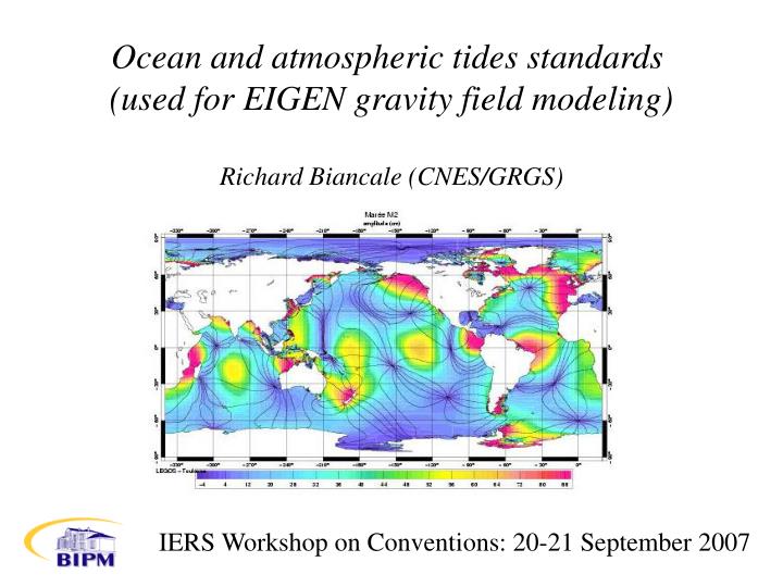
Ocean and atmospheric tides standards (used for EIGEN gravity field modeling) Richard Biancale (CNES/GRGS). IERS Workshop on Conventions: 20-21 September 2007. Ocean tides modeling. The height of ocean tides is expressed by a sum over n waves :. Z n is the amplitude of the wave n ,.

E N D
Ocean and atmospheric tides standards (used for EIGEN gravity field modeling) Richard Biancale (CNES/GRGS) IERS Workshop on Conventions: 20-21 September 2007
Ocean tides modeling The height of ocean tides is expressed by a sum over n waves : Znis the amplitude of the wave n, is the phase is the Doodson argument which is expressed in linear combination of 6 variables : These 6 variables with decreasing frequencies represent the fundamental arguments according to the Sun and Moon motions : τ: angle of the mean lunar day (1.03505 d) s: angle of the mean tropic month (27.32158 d) h: angle of the mean tropic year (365.2422 d) p: angle of the mean lunar perigee (8.8473 y) N‘ : angle of the mean lunar node (18.6129 y) ps : angle of the perihelion (20940.28 y) n1 (= 0, 1, 2, 3...) defines the specie (long period, diurnal, semi-diurnal, ter-diurnal...), n2 the group (in general :1 ≤ n2 ≤ 9) and n3 the constituent (1 ≤ n3 ≤ 9).
The amplitude (Zn) and phase (n) of the different waves of tides represented by cotidal maps can be expanded in spherical harmonic functions of Zncosψn and Znsinψn : Then we have : Writing : the height of tide becomes :
Procedure # reading the point grid by lec_grille(_quart)_degre # converting by gpgm2; point grid C → mean grid C # converting by analhs; mean grid C → alm,blm harmonics # converting by gpgm2; point grid S → mean grid S # converting by analhs; mean grid S → clm,dlm harmonics # converting by convers_hs; (alm,dlm)/(blm,clm) harmonics → Clm±/ Slm± ocean tides harmonics # applying by cor_ellips the ellipsoidal correction
FES2004 Ocean tide model: FES2004 normalized model (fev. 2004) up to (100,100) in cm (long period from FES2002 up to (50,50) + equilibrium Om1/Om2, atmospheric tide NOT included)Doodson l m Csin+ Ccos+ Csin- Ccos- C+ eps+ C- eps- 55.565 Om1 2 0 -0.540594 0.000000 0.000000 0.000000 0.5406 270.000 0.0000 0.000 55.575 Om2 2 0 -0.005218 0.000000 0.000000 0.000000 0.0052 270.000 0.0000 0.000 56.554 Sa 2 0 -0.046604 -0.000903 0.000000 0.000000 0.0466 268.890 0.0000 0.000 57.555 Ssa 2 0 -0.296385 -0.010794 0.000000 0.000000 0.2966 267.914 0.0000 0.000 65.455 Mm 2 0 -0.479140 -0.084083 0.000000 0.000000 0.4865 260.047 0.0000 0.00075.555 Mf 2 0 -0.805539 -0.236132 0.000000 0.000000 0.8394 253.662 0.0000 0.000 85.455 Mtm 2 0 -0.139082 -0.049418 0.000000 0.000000 0.1476 250.439 0.0000 0.000 93.555 Msq 2 0 -0.019391 -0.006674 0.000000 0.000000 0.0205 251.008 0.0000 0.000 135.655 Q1 2 1 -0.291290 0.308134 0.049563 -0.203915 0.4240 316.610 0.2099 166.339145.555 O1 2 1 -1.480706 1.383072 0.455121 -0.792480 2.0262 313.047 0.9139 150.131163.555 P1 2 1 -0.505544 0.551083 0.279251 -0.259244 0.7478 317.468 0.3810 132.872165.555 K1 2 1 -1.530097 1.660923 0.845110 -0.785011 2.2583 317.348 1.1535 132.889 235.755 2N2 2 2 -0.044241 0.134832 0.020987 -0.001671 0.1419 341.834 0.0211 94.552245.655 N2 2 2 -0.577967 0.958489 0.162389 0.009450 1.1193 328.910 0.1627 86.670255.555 M2 2 2 -3.233275 3.840723 0.786314 0.430793 5.0205 319.908 0.8966 61.283273.555 S2 2 2 -1.288610 1.293664 0.040901 0.419782 1.8259 315.112 0.4218 5.565275.555 K2 2 2 -0.337696 0.358821 -0.000662 0.114679 0.4927 316.737 0.1147 359.669 455.555 M4 4 4 -0.000551 -0.003144 0.001155 -0.002202 0.0032 189.949 0.0025 152.313
LAGEOS ocean tides fit over 19 y (normalized coefficients) : LAGEOS FES-2004 difference doodson darw l m C+(cm) ε+(deg) C+(cm) ε+(deg) ΔC+(%) Δε+(%) 55.565 Ω1 2 0 0.4387 223.72 0.5406 270.00 19. 26. 55.575 Ω2 2 0 0.3206 125.05 0.0052 270.00 6044. 80. 56.554 Sa 2 0 0.5800 26.61 0.0466 268.89 1144. 65. 57.555 Ssa 2 0 0.7390 277.17 0.2966 267.91 149. 5. Ω2, Sa and Ssa results are not to be considered in terms of tides but more probably in terms of mass displacement
Admittance function The admittance function is defined for each wave as the ratio between the potential generating tides and the ocean response : with The behavior of the admittance function is smooth in frequency so that it can be interpolated linearly between 2 main waves of close frequencies : with O. Colombo, thesis of S Casotto, (1989)
Comparison of CHAMP orbits over 10 days with the one computed with P1 from FES2004
ELLIPSOIDAL CORRECTIONS TO SPHERICAL HARMONICS OF SURFACE PHENOMENA GRAVITATIONAL EFFECTS Georges Balmino CNES-GRGS 18, Av. Edouard Belin, 31401 TOULOUSE Cedex 9, France georges.balmino@cnes.fr Submitted September 19, 2003 To Technical University of Graz Institut für Geodäsie Special publication in honour of H. Moritz
with with and with
Ellipsoidal correction Model 1: Ocean tide model: FES2004 normalized model (in cm) Model 2: Ocean tide model: FES2004 normalized model with ellipsoidal correction (in cm) model 1 model 2 2 - 1doodson darw l m c+(cm) eps+(deg) c+(cm) eps+(deg.) difference / relative(%) 255.555 M2 1 0 0.5888 40.8014 0.5885 39.9910 -0.0003 -0.8104 0.0 -0.5255.555 M2 2 0 1.2812 180.4369 1.2766 180.0110 -0.0046 -0.4259 -0.4 -0.2255.555 M2 3 0 1.4460 152.1206 1.4422 152.1420 -0.0038 0.0214 -0.3 0.0255.555 M2 4 0 1.6966 295.4730 1.6952 295.3580 -0.0014 -0.1150 -0.1 -0.1255.555 M2 5 0 1.2362 328.6181 1.2222 328.0520 -0.0140 -0.5661 -1.1 -0.3255.555 M2 1 1 0.3929 140.8622 0.3979 141.2420 0.0050 0.3798 1.3 0.2255.555 M2 2 1 1.0510 250.4822 1.0551 250.0190 0.0041 -0.4632 0.4 -0.3255.555 M2 3 1 1.2578 345.4651 1.2555 346.4350 -0.0023 0.9699 -0.2 0.5255.555 M2 4 1 2.3442 30.4333 2.3297 30.3530 -0.0145 -0.0803 -0.6 0.0255.555 M2 5 1 3.5506 237.7274 3.5192 237.7810 -0.0314 0.0536 -0.9 0.0255.555 M2 2 2 5.0115 319.9495 5.0205 319.9080 0.0090 -0.0415 0.2 0.0255.555 M2 3 2 0.8508 171.8101 0.8549 172.0060 0.0041 0.1959 0.5 0.1255.555 M2 4 2 4.7345 128.8852 4.7241 129.0010 -0.0104 0.1158 -0.2 0.1255.555 M2 5 2 1.7639 9.9130 1.7569 9.9690 -0.0070 0.0560 -0.4 0.0255.555 M2 3 3 3.2388 36.5296 3.2347 36.7060 -0.0041 0.1764 -0.1 0.1255.555 M2 4 3 3.7611 178.5463 3.7461 178.4950 -0.0150 -0.0513 -0.4 0.0255.555 M2 5 3 2.8611 295.8639 2.8309 295.7940 -0.0302 -0.0699 -1.1 0.0255.555 M2 4 4 3.7494 302.6906 3.7439 302.6140 -0.0055 -0.0766 -0.1 0.0255.555 M2 5 4 4.0702 49.1312 4.0430 49.1210 -0.0272 -0.0102 -0.7 0.0255.555 M2 5 5 0.8065 70.9801 0.8011 70.6670 -0.0054 -0.3131 -0.7 -0.2
GRGS-GRACE tide model Model 1 : Ocean tide model: FES2004 normalized model (fev. 2004) up to (100,100) in cm (long period from FES2002 up to (50,50) + equilibrium Om1/Om2, atmospheric tide Model 2 : OCEAN TIDES – from GRACE solution model 1 model 2 2 - 1 doodson l m c+(cm) eps+(deg) c+(cm) eps+(deg.) difference / relative(%)135.655 Q1 2 1 0.4240 316.6096 0.4603 313.7090 0.0363 -2.9006 8.6 -1.6145.555 O1 2 1 2.0262 313.0474 1.9586 315.2550 -0.0676 2.2076 -3.3 1.2163.555 P1 2 1 0.7478 317.4678 0.6771 316.2990 -0.0707 -1.1688 -9.5 -0.6165.555 K1 2 1 2.2583 317.3477 2.4783 323.8800 0.2200 6.5323 9.7 3.6 235.755 2N2 2 2 0.1419 341.8343 0.1484 338.2020 0.0065 -3.6323 4.6 -2.0245.655 N2 2 2 1.1193 328.9101 1.1100 330.6140 -0.0093 1.7039 -0.8 0.9255.555 M2 2 2 5.0205 319.9080 4.8235 321.1620 -0.1970 1.2540 -3.9 0.7273.555 S2 2 2 1.8259 315.1121 1.8941 309.9170 0.0682 -5.1951 3.7 -2.9275.555 K2 2 2 0.4927 316.7372 0.2573 311.0220 -0.2354 -5.7152 -47.8 -3.2
Temporal evolution of the geoid differences derived from the mean atmospheric tide models based on 6h ECMWF pressure field data (1985-2002) for August 2, each 3h. 0h 3h 6h 9h 12h 15h 18h 21h
S1 S2 ECMWF derived atmospheric tides (Bode & Biancale,2003) normalized model (in mbar) Doodson Darw l m Csin+ Ccos+ C+ eps+ 164.556 S1 0 0 -0.010427 0.004887 0.0115 295.112 164.556 S1 1 0 -0.011572 0.007151 0.0136 301.714 164.556 S1 2 0 -0.021999 -0.019367 0.0293 228.641 164.556 S1 3 0 -0.019447 -0.001090 0.0195 266.792 164.556 S1 1 1 0.211548 0.063876 0.2210 73.199 164.556 S1 2 1 0.011431 0.014826 0.0187 37.633 164.556 S1 3 1 -0.125362 -0.011301 0.1259 264.849 164.556 S1 4 1 0.006730 -0.015007 0.0164 155.846 164.556 S1 2 2 0.040451 0.052284 0.0661 37.728 164.556 S1 3 2 -0.000839 0.024861 0.0249 358.067 164.556 S1 4 2 -0.027001 -0.014535 0.0307 241.706 164.556 S1 5 2 0.001710 -0.002672 0.0032 147.382 164.556 S1 3 3 -0.016213 -0.011110 0.0197 235.579 164.556 S1 4 3 -0.028287 0.015258 0.0321 298.342 164.556 S1 5 3 -0.018513 -0.003835 0.0189 258.297 164.556 S1 6 3 -0.001229 -0.011130 0.0112 186.301 164.556 S1 4 4 -0.011813 0.026961 0.0294 336.339 164.556 S1 5 4 0.013651 -0.002437 0.0139 100.122 164.556 S1 6 4 0.005458 0.007862 0.0096 34.769 164.556 S1 7 4 -0.002848 0.010407 0.0108 344.695 164.556 S1 5 5 -0.019909 0.031089 0.0369 327.365 164.556 S1 6 5 0.034243 -0.001804 0.0343 93.016 164.556 S1 7 5 0.011923 0.001275 0.0120 83.896 164.556 S1 8 5 -0.006841 -0.000462 0.0069 266.136 ECMWF derived atmospheric tides (Bode & Biancale,2003) normalized model (in mbar) Doodson Darw l m Csin+ Ccos+ C+ eps+ 273.555 S2 0 0 -0.001267 0.004729 0.0049 345.001 273.555 S2 1 0 0.003017 -0.001218 0.0033 111.985 273.555 S2 2 0 0.046910 -0.110495 0.1200 156.997 273.555 S2 3 0 0.011240 0.003652 0.0118 72.000 273.555 S2 1 1 0.025133 -0.003030 0.0253 96.874 273.555 S2 2 1 0.011672 -0.022752 0.0256 152.842 273.555 S2 3 1 -0.019507 0.009509 0.0217 295.988 273.555 S2 4 1 -0.004188 0.001154 0.0043 285.406 273.555 S2 2 2 0.283369 -0.468298 0.5474 148.822 273.555 S2 3 2 0.009812 0.026639 0.0284 20.220 273.555 S2 4 2 -0.036313 0.070506 0.0793 332.750 273.555 S2 5 2 -0.004402 -0.002872 0.0053 236.878 273.555 S2 3 3 0.016795 0.005516 0.0177 71.818 273.555 S2 4 3 0.003813 -0.000086 0.0038 91.292 273.555 S2 5 3 -0.004878 0.006430 0.0081 322.815 273.555 S2 6 3 0.001879 0.001580 0.0025 49.940 273.555 S2 4 4 -0.015098 0.000828 0.0151 273.139 273.555 S2 5 4 0.002428 0.008129 0.0085 16.630 273.555 S2 6 4 -0.001503 0.000413 0.0016 285.365 273.555 S2 7 4 -0.004306 -0.001009 0.0044 256.812 273.555 S2 5 5 0.009324 -0.000794 0.0094 94.867 273.555 S2 6 5 0.000304 0.000524 0.0006 30.120 273.555 S2 7 5 0.003957 -0.000054 0.0040 90.782 273.555 S2 8 5 0.005283 0.001430 0.0055 74.854
Sa Ssa ECMWF derived atmospheric tides (Bode & Biancale,2003) normalized model (in mbar) Doodson Darw l m Csin+ Ccos+ C+ eps+ 56.554 Sa 0 0 -0.168856 -0.049683 0.1760 253.604 56.554 Sa 1 0 0.105071 -0.057879 0.1200 118.848 56.554 Sa 2 0 0.071952 0.653729 0.6577 6.281 56.554 Sa 3 0 -1.225490 -0.371665 1.2806 253.129 56.554 Sa 1 1 0.047282 0.220890 0.2259 12.082 56.554 Sa 2 1 0.306172 0.548859 0.6285 29.154 56.554 Sa 3 1 -0.042330 0.336106 0.3388 352.822 56.554 Sa 4 1 -0.112705 -0.170263 0.2042 213.502 56.554 Sa 2 2 -0.218981 0.158912 0.2706 305.968 56.554 Sa 3 2 -0.256851 -0.042370 0.2603 260.633 56.554 Sa 4 2 -0.264284 0.003188 0.2643 270.691 56.554 Sa 5 2 -0.197183 -0.006217 0.1973 268.194 56.554 Sa 3 3 0.133799 -0.031722 0.1375 103.338 56.554 Sa 4 3 0.096020 0.241783 0.2602 21.660 56.554 Sa 5 3 0.181815 0.111700 0.2134 58.435 56.554 Sa 6 3 0.017368 0.156099 0.1571 6.349 56.554 Sa 4 4 0.013902 -0.131590 0.1323 173.969 56.554 Sa 5 4 -0.103664 -0.034022 0.1091 251.830 56.554 Sa 6 4 0.061234 -0.034274 0.0702 119.237 56.554 Sa 7 4 -0.053530 0.014686 0.0555 285.342 56.554 Sa 5 5 -0.013892 -0.035348 0.0380 201.455 56.554 Sa 6 5 0.093559 -0.112805 0.1466 140.328 56.554 Sa 7 5 0.056152 -0.089431 0.1056 147.876 56.554 Sa 8 5 0.047282 -0.034263 0.0584 125.929 ECMWF derived atmospheric tides (Bode & Biancale,2003) normalized model (in mbar) Doodson Darw l m Csin+ Ccos+ C+ eps+ 57.555 Ssa 0 0 0.026418 -0.043967 0.0513 149.000 57.555 Ssa 1 0 0.213356 0.369254 0.4265 30.019 57.555 Ssa 2 0 -0.037297 0.093489 0.1007 338.251 57.555 Ssa 3 0 0.440373 0.198389 0.4830 65.748 57.555 Ssa 1 1 -0.187842 -0.054635 0.1956 253.783 57.555 Ssa 2 1 -0.100279 0.028146 0.1042 285.678 57.555 Ssa 3 1 0.022220 0.062821 0.0666 19.479 57.555 Ssa 4 1 0.025233 0.041395 0.0485 31.365 57.555 Ssa 2 2 -0.033028 0.012868 0.0354 291.286 57.555 Ssa 3 2 -0.071309 0.002881 0.0714 272.314 57.555 Ssa 4 2 0.028970 0.007771 0.0300 74.984 57.555 Ssa 5 2 -0.028689 -0.015389 0.0326 241.791 57.555 Ssa 3 3 -0.075016 -0.066689 0.1004 228.363 57.555 Ssa 4 3 0.007825 -0.056142 0.0567 172.065 57.555 Ssa 5 3 -0.111399 -0.068246 0.1306 238.507 57.555 Ssa 6 3 -0.022692 -0.077537 0.0808 196.313 57.555 Ssa 4 4 -0.003236 -0.013119 0.0135 193.856 57.555 Ssa 5 4 0.048517 -0.037387 0.0613 127.618 57.555 Ssa 6 4 -0.013902 0.014806 0.0203 316.804 57.555 Ssa 7 4 0.035921 0.013320 0.0383 69.655 57.555 Ssa 5 5 0.004073 -0.025976 0.0263 171.089 57.555 Ssa 6 5 0.000599 -0.026941 0.0269 178.726 57.555 Ssa 7 5 -0.037086 -0.009590 0.0383 255.502 57.555 Ssa 8 5 -0.028427 -0.007664 0.0294 254.912
Comparison to the Haurwitz and Cowley model Model 1 : H & W atmospheric tides (Haurwitz & Cowley, 1973) normalized model up to (8,5) (in mbar) Model 2 : ECMWF derived atmospheric tides (Bode & Biancale, 2003) normalized model up to (8,5) (in mbar) model 1 model 2 2 - 1 doodson l m c+(mb) eps+(deg) c+(mb) eps+(deg.) difference / relative(%)164.556 S1 1 1 0.2885 12.0001 0.2210 73.1990 -0.0675 61.1989 -23.4 34.0164.556 S1 2 1 0.0365 330.9997 0.0187 37.6330 -0.0178 66.6333 -48.8 37.0164.556 S1 3 1 0.0860 197.0001 0.1259 264.8490 0.0399 67.8489 46.4 37.7 273.555 S2 2 2 0.5510 159.0000 0.5474 148.8220 -0.0036 -10.1780 -0.7 -5.7273.555 S2 3 2 0.0260 81.0007 0.0284 20.2200 0.0024 -60.7807 9.2 -33.8273.555 S2 4 2 0.0540 330.9995 0.0793 332.7500 0.0253 1.7505 46.9 1.0