Download
1 / 20
200 likes | 285 Views
Consistency between the flow at the top of the core and the frozen-flux approximation. Kathy Whaler, University of Edinburgh Richard Holme, Liverpool University. Background. Induction equation in the frozen-flux approximation. Some flow information can be derived directly from this:

E N D
Consistency between the flow at the top of the core and the frozen-flux approximation Kathy Whaler, University of Edinburgh Richard Holme, Liverpool University
Background Induction equation in the frozen-flux approximation Some flow information can be derived directly from this: (i) At local extrema of Br (ii) On null-flux curves, NFC (contours on which Br=0) where v1 is the flow component perpendicular to the NFC
Tests • Are flows calculated by inverting the induction equation consistent with the direct information? • How much are the flows modified if the direct information is imposed as side constraints during inversion? • How do we calculate the uncertainties on the various quantities involved?
Method • Use the ufm model of Bloxham and Jackson (1992) for 1970-1980 • Invert secular variation coefficients at 1970, 1975 and 1980 for a steady flow (also a tangentially geostrophic flow for 1980) • Approximately 75 extrema at each epoch • Find a similar number of points along NFCs • Compare direct and inverted values of H.v and v1
Extrema comparisons Comparison between and (in nT/yr) at the extrema of Br. Left hand set of columns is for a damping parameter of 5 x 10⁻⁵, the right hand set for 10-4.
NFC comparisons Comparison between rms values of v1 (in km/yr) on NFCs. Left hand steady flow columns for a damping parameter of 5 x 10⁻⁵, right hand for 10-5. For the 1980 tangentially geostrophic flow, damping parameters are 10-3 (left) and 10-5 (right).
Summary • Differences between direct and inversion estimates of quantities are as large as the quantities themselves • Suggests inversion flows are incompatible with underlying frozen-flux assumptions • Can small changes to the inversion flow pattern bring it into agreement?
Imposing frozen-flux constraints • Add as side constraints using a Lagrange multiplier • Constrain at extrema rather than • When satisfied at the 90% level, fit to the secular variation coefficients is considerably degraded, and complexity of the flow significantly increased
Both constraints simultaneously • Very difficult to satisfy both sets of constraints simultaneously • Consider small null-flux patch beneath the North Atlantic • Both Br and are positive within it, implying convergence • But, on the NFC bounding it, because is positive, the flow is anti-parallel to , i.e. outward, and hence divergent • Quantify uncertainties to assess how serious discrepancies are
Uncertainties • rms uncertainty on depends strongly on truncation level • 1381 nT/yr for degree 10, 17493 nT/yr for degree 14; take 1500 nT/yr as representative • rms uncertainty on is 207 nT/km for degree 14 – many extrema not well constrained • Two uncertainties combined at the 1 standard deviation level – constraints fail at only 5 out of 75 extrema, well below 1/3 expected by chance • Uncertainty on Br significantly smaller than on other quantities
Grey shaded areas enclose 1 standard deviation uncertainties on extremal positions; contours are ± 500, 1000 and 1500 nT/yr of . Thus grey shaded areas should be cut by a contour.
Flow component uncertainties • Several sources of uncertainty • On the direct value of v1 - calculate pointwise • On the direction of the normal to the NFC – can’t straightforwardly calculate an rms value, so estimate its standard deviation at individual points • Very variable, depending on how ‘flat’ Br is at the point • On the flow components obtained from inversion – use the covariance matrix
Flow component uncertainties Component of inversion flow in direction of v1 and its uncertainty All inverse flow components within green cone possible v1 Inversion flow and its error ellipse NFC
Summary v1 NFC results • Approximately 2/3 of the unconstrained inversion flow components match the direct components to within the sum of the various uncertainties • Almost all the NFC constrained flow components match the direct components • Only about 40% of the extremal constrained flow components match the direct components
Summary • Differences between aspects of the direct and (unconstrained) inverse flow are within the uncertainties • No need to build constraints into inversion • ufm field model used here is not itself consistent with frozen-flux – may be affecting results • Newer satellite based models may reduce the secular variation, and hence flow, uncertainties