Download
1 / 21
210 likes | 316 Views
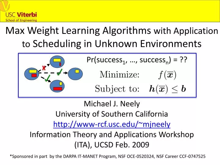
Max Weight Learning Algorithms with Application to Scheduling in Unknown Environments. Pr(success 1 , …, success n ) = ??. Michael J. Neely University of Southern California http://www-rcf.usc.edu/~mjneely Information Theory and Applications Workshop (ITA), UCSD Feb. 2009.

E N D
Max Weight Learning Algorithms with Application to Scheduling in Unknown Environments Pr(success1, …, successn) = ?? Michael J. Neely University of Southern California http://www-rcf.usc.edu/~mjneely Information Theory and Applications Workshop (ITA), UCSD Feb. 2009 *Sponsored in part by the DARPA IT-MANET Program, NSF OCE-0520324, NSF Career CCF-0747525
5 6 0 1 2 3 4 • Slotted System, slots t in {0, 1, 2, …} • Network Queues: Q(t) = (Q1(t), …, QL(t)) • 2-Stage Control Decision Every slot t: • 1) Stage 1 Decision: k(t) in {1, 2, …, K}. • Reveals random vector w(t) (iid given k(t)) • w(t) has unknown distribution Fk(w). • 2) Stage 2 Decision:I(t) in I(a possibly infinite set). • Affects queue rates: • A(k(t), w(t), I(t)) , m(k(t), w(t),I(t)) • Incurs a “Penalty Vector” x(t): • x(t) = x(k(t), w(t), I(t))
Stage 1: k(t) in {1, …, K}. Reveals random w(t). Stage 2: I(t) in I. Incurs Penalties x(k(t), w(t), I(t)). Also affects queue dynamics A(k(t), w(t), I(t)) , m(k(t), w(t),I(t)). Goal: Choose stage 1 and stage 2 decisions over time so that the time average penalties x solve: f(x), hn(x) general convex functions of multi-variables
Motivating Example 1: Min Power Scheduling with Channel Measurement Costs S1(t) A1(t) Minimize Avg. Power Subject to Stability S2(t) A2(t) AL(t) SL(t) If channel states are known every slot: Can Schedule without knowing channel statistics or arrival rates! (EECA --- Neely 2005, 2006) (Georgiadis, Neely, Tassiulas F&T 2006)
Motivating Example 1: Min Power Scheduling with Channel Measurement Costs S1(t) A1(t) Minimize Avg. Power Subject to Stability S2(t) A2(t) AL(t) SL(t) If “cost” to measuring, we make a 2-stage decision: Stage 1: Measure or Not? (reveals channels w(t) ) Stage 2: Transmit over a known channel? a blind channel? -Li and Neely (07) -Gopalan, Caramanis, Shakkottai (07) Existing Solutions require a-priori knowledge of the full joint-channel state distribution! (2L , 1024L ? )
Motivating Example 2: Diversity Backpressure Routing (DIVBAR) 3 2 error 1 [Neely, Urgaonkar 2006, 2008] broadcasting Networking with Lossy channels & Multi-Receiver Diversity: DIVBAR Stage 1: Choose Commodity and Transmit DIVBAR Stage 2: Get Success Feedback, Choose Next hop If there is a single commodity (no stage 1 decision), we do not need success probabilities! If two or more commodities, we need full joint success probability distribution over all neighbors!
Stage 1: k(t) in {1, …, K}. Reveals random w(t). Stage 2: I(t) in I. Incurs Penalties x(k(t), w(t), I(t)). Also affects queue dynamics A(k(t), w(t), I(t)) , m(k(t), w(t),I(t)). Goal: Equivalent to: Where g(t) is an auxiliary vector that is a proxy for x(t).
Stage 1: k(t) in {1, …, K}. Reveals random w(t). Stage 2: I(t) in I. Incurs Penalties x(k(t), w(t), I(t)). Also affects queue dynamics A(k(t), w(t), I(t)) , m(k(t), w(t),I(t)). Equivalent Goal: Technique: Form virtual queues for each constraint. U(t) b h(g(t)) Un(t+1) = max[Un(t) + hn(g(t)) – bn,0] Z(t) x(t) g(t) Zm(t+1) = Zm(t) – gm(t) + xm(t) Possibly negative
Use Stochastic Lyapunov Optimization Technique: [Neely 2003], [Georgiadis, Neely, Tassiulas F&T 2006] Define: Q(t) = All Queues States = [Q(t), Z(t), U(t)] Define: L(Q(t)) = (1/2)[sum of squared queue sizes] Define: D(Q(t)) = E{L(Q(t+1)) – L(Q(t))|Q(t)} Schedule using the modified “Max-Weight” Rule: Every slot t, observe queue states and make a 2-stage decision to minimize the “drift plus penalty”: Minimize:D(Q(t)) + Vf(g(t)) Where V is a constant control parameter that affects Proximity to optimality (and a delay tradeoff).
How to (try to) minimize: Minimize:D(Q(t)) + Vf(g(t)) The proxy variables g(t) appear separably, and their terms can be minimized without knowing system stochastics! Minimize: Subject to: [Zm(t) and Un(t) are known queue backlogs for slot t]
Minimizing the Remaining Terms: Minimize:D(Q(t)) + Vf(g(t))
Solution: Defineg(mw)(t), I(mw)(t) , k(mw)(t) as the ideal max-weight decisions (minimizing the drift expression). Define ek(t): Then: ? k(mw)(t) = argmin{k in {1,.., K}} ek(t) (Stage 1) I(mw)(t) = argmin{I in I} Yk(t)(w(t), I, Q) (Stage 2) g(mw)(t) = solution to the proxy problem
Approximation Theorem: (related to Neely 2003, G-N-T F&T 2006) If actual decisions satisfy: With: (related to slackness of constraints) Then: -All Constraints Satisfied. [B + C + c0V] min[emax – eQ, s – eZ] -Average Queue Sizes < -Penalty Satisfies: f( x ) < f*optimal + O(max[eQ,eZ]) + (B+C)/V
It all hinges on our approximation of ek(t): Declare a “type k exploration event” independently with probability q>0 (small). We must use k(t) = k here. Approach 1: {w1(k)(t), …, wW(k)(t)} = samples over past W type kexplor. events
It all hinges on our approximation of ek(t): Declare a “type k exploration event” independently with probability q>0 (small). We must use k(t) = k here. Approach 2: {w1(k)(t), …, wW(k)(t)} = samples over past W type kexplor. Events {Q1(k)(t), …, QW(k)(t)} = queue backlogs at these sample times.
Analysis (Approach 2): Subtleties: “Inspection Paradox” issue requires use of samples at exploration events, so {w1(k)(t), …, wW(k)(t)} iid. 2) Even so, {w1(k)(t), …, wW(k)(t)} are correlated with queue backlogs at time t, and so we cannot directly apply the Law of Large Numbers!
Analysis (Approach 2): w1(t) w2(t) w3(t) wW(t) tstart t Use a “Delayed Queue” Analysis: Can Apply LLN constant constant
Max-Weight Learning Algorithm (Approach 2): (No knowledge of probability distributions is required!) -Have Random Exploration Events (prob. q). -Choose Stage-1 decision k(t) = argmin{k in {1,.., K}}[ ek(t) ] -Use I(mw)(t) for Stage-2 decision: I(mw)(t) = argmin{I in I} Yk(t)(w(t), I, Q(t)) -Use g(mw)(t) for proxy variables. -Update the virtual queues and the moving averages.
Theorem (Fixed W, V): With window size W we have: -All Constraints Satisfied. [B + C + c0V] min[emax – eQ, s – eZ] -Average Queue Sizes < -Penalty Satisfies: f( x ) < f*q + O(1/sqrt{W}) + (B+C)/V
Concluding Theorem (Variable W, V): Let 0 < b1 < b2 < 1. Define V(t) = (t + 1) b1 , W(t) = (t+1)b2 Then under the Max-Weight Learning Algorithm: -All Constraints are Satisfied. -All Queues are mean rate stable*: -Average Penalty gets exact optimality (subject to random exploration events): *Mean rate stability does not imply finite average congestion and delay. In fact, Average congestion and delay are necessarily infinite when exact optimality is reached. f( x ) = f*q