Download
1 / 32
320 likes | 440 Views
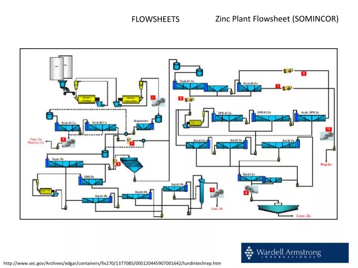
Zinc Plant Flowsheet (SOMINCOR). FLOWSHEETS. http://www.sec.gov/Archives/edgar/containers/fix270/1377085/000120445907001642/lundintechrep.htm. Analysis of flowsheets. SIMPLE CASE. final tailing. final concentrate. Balance of each node. GRADE . – content of a component in feed %,

E N D
Zinc Plant Flowsheet (SOMINCOR) FLOWSHEETS http://www.sec.gov/Archives/edgar/containers/fix270/1377085/000120445907001642/lundintechrep.htm
Analysis of flowsheets SIMPLE CASE finaltailing finalconcentrate
Balance of eachnode GRADE – content of a component in feed %, – content of a component in concentrate, %, – content of a component in combined products, %, – content of a component in tailing, % Input data inputparameters: α, , calculatedparameteres: , , r, a… – yield of a product , % – recoveryof a considered component in a product, % r– recoveryof otherthanconsideredcomponents in anotherproduct, % *, and r calculated from α,, semiproduct P1 feed α concetrate tailing concentrate C1 concentrate C2
EQUATIONS (%) (%) (%) (-) a = 100 idealseparation , a ~ 1000 no separation
feed product grade ,% F 1.421 100.0 100.0 yield,% recov., % 1 P1 15.25 P2 0.2185 8.00 85.85 92.00 14.15 2 3 C2 7.000 T 0.150 C1 29.00 C3 0.60 62.50 28.69 84.8458.20 37.5071.31 15.2241.80 tailing T concentrate C3 concentrate C2 concentrate C1 Flowsheet with balances of nodes (localbalances)
Upgradingcurves for nodesusinglocalbalances conclusion: separationisbest in node 1 (a=101.30 and worse in nodes 2 and 3, a=~125)
Best flotation results upgrading curve EQUATIONS weightedaverage for instance for products C1+C2
Feed 1 semiproduct P2 semiproduct P1 concentrate C1 2 3 concentrate C2 tailing T concentrate C3 4 final concentrate Cf final tailing T f Options of industrialflowsheet
Feed Feed 1 semiproduct P2 semiproduct P1 1 semiproduct P2 semiproduct P1 concentrate C1 2 3 concentrate C2 tailing T concentrate C3 2 3 5 final concentrate C final tailing T 4 f f final concentrate C final tailing T f f = =
Feed 1 semiproduct P2 semiproduct P1 concentrate C1 2 3 concentrate C2 tailing T concentrate C3 4 final concentrate C final tailing T f f
Feed 1 semiproduct P2 semiproduct P1 concentrate C1 2 3 concentrate C2 tailing T concentrate C3 5 4 final concentrate C final tailing T f f
Feed 1 semiproduct P2 semiproduct P1 concentrate C1 2 3 concentrate C2 tailing T concentrate C3 4 final concentrate C final tailing T f f
Selectivity of separation for differentoptions of composition of finalflotation products =
Selection of optimum point of process commonsense optimum point of separation example of point of optimum separationbased on economics Finaldecision: Cf=C1+C2 + somethingdepending on criterion of upgradingoptimal point
Transformation of the Fuerstenau(recovery-recoveryor-)upgradingcurveinto Halbich (grade-recoveryorβ- ) upgradingcurve the Fuerstenau (-)is alfa -insensitiveequivalent of the Halbich (β- ) upgradingcurve
Flowsheet with balance of nodes (localbalances) inputparameters: α, ,
EQUATIONS Recyclenode (1) Separatingnodes (%) (%) (%) (-) a = 100 idealseparation , a ~ 1000 no separation
node l g S g e S e e 2 r 0,00 0,00 100,00 25,00 0,89 0,89 28,40 28,40 99,33 0,57 99,11 100,00 71,60 100,00 0,00 0,78 l g S g e S e e 4 r 0,00 0,00 100,00 25,00 11,76 11,76 52,63 52,63 90,65 3,00 88,24 100,00 47,37 100,00 0,00 5,59 l g S g e S e e 5 r 0,00 0,00 100,00 0,60 78,48 78,48 83,30 83,30 21,55 0,44 21,52 100,00 16,70 100,00 0,00 0,57
Upgradingcurves for nodesusinglocalbalances node 5 is not efficient
Global balance of flowsheet(feed F2 is 100%) knownparameters: α, , Eqs for recycling nodes
Calculations Feed 1: gradesareknown, G and Gareequal to 100% Node 1 Gradesareknown, local and for F1 areknown (=21.95%) (for C3 is 100- 21.95 =78.05%) orcan be calculated from grades of products Calculation of global for F2 Q) How largeis for C3 when for F1 is 100%? A) WhenF1=100%, C3 =(100/21.95)x 78.05= 350%. Then F2= F1+C3 = 100+350=450%
Graphicalrepresentation of separation data (not veryuseful, recoveriesgreaterthan 100%) Grade –recoverycurve for Pb, Cu and Zn circuitswithin the Eureka Concentrator (based on Ch. Greet, Spectrum Series, 2010)
The Eureka Mine – An Example of How to Identify andSolve Problems in a Flotation Plant Christopher Greet
Usefulliterature The Eureka Mine – An Example of How to Identify andSolve Problems in a Flotation Plant Christopher Greet
Homework Createyourownflowsheet and calculatelocal and globalbalanses as well as plot graphswhichwillhelpyou to evaluate the plant performance