Download

1 / 25
250 likes | 398 Views
Dynamic trees (Steator and Tarjan 83). Operations that we do on the trees. Maketree(v) w = findroot(v) (v,c) = mincost(v) addcost(v,c) link(v,w,r(v,w)) cut(v) findcost(v). Definitions. We represent each tree T by a virtual tree V. The virtual tree is a binary tree with middle children.

E N D
Operations that we do on the trees Maketree(v) w = findroot(v) (v,c) = mincost(v) addcost(v,c) link(v,w,r(v,w)) cut(v) findcost(v)
Definitions • We represent each tree T by a virtual tree V. The virtual tree is a binary tree with middle children. left middle right Think of V as partitioned into solid subtrees connected by dashed edges What is the relation between V and T ?
d f g i l j Actual tree a b c e h k p q m n o r s t u v w
d f g i j l Path decomposition a Partition T into disjoint paths b c e h k p q m n o r s t u v w
Virtual trees (cont) Each path in T corresponds to a solid subtree in V f l b q c i a p j h The parent of a vertex x in T is the successor of x (in symmetric order) in its solid subtree or the parent of the solid subtree if x is the last in symmetric order in this subtree r g e k m d o n v w t u s
f d i g j l Virtual trees (cont) f a l b b q c i a c p e j h h r g e k k p q m d m n o o n v r s t w t u u s v w
Virtual trees (representation) Each vertex points to p(x) to its left son l(x) and to its right son r(x). A vertex can easily decide if it is a left child a right child or a middle child. Each solid subtree functions like a splay tree.
a b c d e f Simple case -- paths Assume for a moment that each tree T in the forest is a path so each virtual tree is a simple splay tree. d b e a c f
Findroot(v) Splay at v, then follow right pointers until you reach the last vertex w on the right path. Return w and splay at w.
1 4 3 2 7 a b c d e f Mincost(v) With every vertex x we record cost(x) = the cost of the edge (x,p(x)) We also record with each vertex x mincost(x) = minimum of cost(y) over all descendants y of x. 7,1 d 3,1 4,4 b e 2,2 1,1 , a c f
Mincost(v) Splay at v and use mincost values to search for the minimum Notice: we need to update mincost values as we do rotations. y x x C A y B C A B
1 4 3 2 7 a b c d e f Addcost(v,c) Rather than storing cost(x) and mincost(x) we will store cost(x) = cost(x) - cost(p(x)) min(x) = cost(x) - mincost(x) Addcost(v,c) : Splay at v, cost(v) += c cost(left(v)) -= c similarly update min 7,7,6 d 3,-4,2 4,-3,0 b e 2,-1,0 1,-2,0 , , 0 a c f
Addcost(v,c) (cont) Notice that now we have to update cost(x) and min(x) through rotations w v v C A w b b B C A B cost’(v) = cost(v) + cost(w) cost’(w) = -cost(v) cost’(b) = cost(v) + cost(b)
Addcost(v,c) (cont) Update min: w v v C A w b b B C A B min’(w) = max{0, min(b) - cost’(b), min(c) - cost(c)} min’(v) = max{0, min(a) - cost(a), min’(w) - cost’(w)}
Link(v,w,c), cut(v) Translate directly into catenation and split of splay trees if we talk about paths. Lets do the general case now.
The general case Each solid subtree of a virtual tree is a splay tree. We represent costs essentially as before. cost(x) = cost(x) - cost(p(x)) or cost(x) is x is a root of a solid subtree min(x) = cost(x) - mincost(x) (where mincost is the minimum cost within the subtree)
Splicing Want to change the path decomposition such that v and the root are on the same path. Let w be the root of a solid subtree and v a middle child of w w w ==> right right u v v u Want to make v the left child of w. It requires: cost’(v) = cost(v) - cost(w) cost’(u) = cost(u) + cost(w) min’(w) = max{0, min(v) - cost’(v), min(right(w))- cost(right(w))}
v v Splicing (cont) What is the effect on the path decomposition of the real tree ? w w ==> right right u v v u a a ==> b b w w u u
After the first pass the path from x to the root consists entirely of dashed edges v w x Splaying the virtual tree Let x be the vertex in which we splay. We do 3 passes: 1) Walk from x to the root and splay within each solid subtree 2) Walk from x to the root and splice at each proper ancestor of x. Now x and the root are in the same solid subtree 3) Splay at x Now x is the root of the entire virtual tree.
Dynamic tree operations w = findroot(v) : Splay at v, follow right pointers until reaching the last node w, splay at w, and return w. (v,c) = mincost(v) : Splay at v and use cost and min to follow pointer to the smallest node after v on its path (its in the right subtree of v). Let w be this node, splay at w. addcost(v,c) : Splay at v, increase cost(v) by c and decrease cost(left(v)) by c, update min(v) link(v,w,r(v,w)) : Splay at v and splay at w and make v a middle child of w cut(v) : Splay at v, break the link between v and right(v), set cost(right(v)) += cost(v)
Dynamic tree (analysis) It suffices to analyze the amortized time of splay. An extension of the access lemma. Recall: Assign weight 1 to each node. The size of a node is the total number of descendants it has in the virtual tree. Rank is the log of the size. Change: Potential is c+1 times the sum of the ranks for some constant c. The access lemma then shows that the amortized cost of the splay is 3(r(root)-r(x)) + 1 - 2c L/2 where L is the length of the splay path. This is at most clogn +1 - c(L-1). pass 1 takes 3clogn + k pass 2 takes k pass 3 takes 3clogn + 1 - c(k-1) k=#dashed edges on the path For an appropriate c this is O(log n)
Proof of the access lemma (cont) (3) zig y x ==> x C A y B C A B amortized time(zig) = 1 + = 1 + r’(x) + r’(y) - r(x) - r(y) 1 + r’(x) - r(x) 1 + 3(r’(x) - r(x))
z y D C x A B Proof of the access lemma (cont) (1) zig - zig x ==> A y B z C D amortized time(zig) = 1 + = 2 + r’(x) + r’(y) + r’(z) - r(x) - r(y) - r(z) = 2 + r’(y) + r’(z) - r(x) - r(y) 2 + r’(x) + r’(z) - 2r(x) 2r’(x) - r(x) - r’(z) + r’(x) + r’(z) - 2r(x) = 3(r’(x) - r(x))
Proof of the access lemma (cont) (2) zig - zag z x ==> y D y z A B C D x A B C Similar. (do at home)