Download
1 / 19

E N D
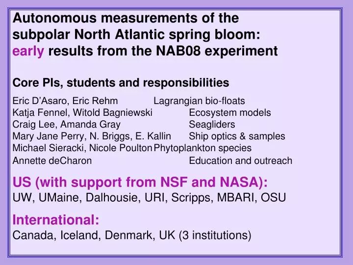
Autonomous measurements of the subpolar North Atlantic spring bloom: early results from the NAB08 experimentCore PIs, students and responsibilitiesEric D’Asaro, Eric Rehm Lagrangian bio-floatsKatja Fennel, Witold Bagniewski Ecosystem models Craig Lee, Amanda Gray SeaglidersMary Jane Perry, N. Briggs, E. Kallin Ship optics & samplesMichael Sieracki, Nicole Poulton Phytoplankton species Annette deCharon Education and outreachUS (with support from NSF and NASA):UW, UMaine, Dalhousie, URI, Scripps, MBARI, OSUInternational:Canada, Iceland, Denmark, UK (3 institutions)
OCB Theme II : Carbon uptake, removal and storage So, why the subpolar North Atlantic ?Carbon uptake:One of largest CO2 draw-downs on the planet occurs during NA spring bloom –> photosynthetic uptake of carbonCarbon Removal: 3 mechanisms * mixed-layer pump (stratification/destratification) * sinking of aggregates (diatoms, etc.) * subduction of water massCarbon Storage:depends on – how much gets down, how fast, and what happens next . . .
Key OCB questions: 1) how much carbon is taken up ? 2) how much carbon is removed ? 3) how much carbon is stored ? 4) how will carbon uptake, removal and storage in the N. Atlantic, and other key regions, respond to climate changeor increased variability in forcings ? 5) how can one document change – in light oflarge temporal and spatial variability ?
Aqua MODIS 24June08 Challenges to studying NA bloom (and other regions) High spatial variability on mesoscale and submesoscale (~ km) Inter-annual variability in timing of bloom (1D model, similar to SeaWiFS data)
Challenges to assessing carbon uptake and removal: Ships – operate on fixed schedules (match or mismatch with timing of the bloom and major removal events)Moorings – single locations, how to interpret submesocale variability ?Satellites – can’t see through (persistent) clouds; lack depth resolutionModels – depend on quality of input data and understanding of processes
Approach: * autonomous 4-D sampling for 3 month, April–June * 2 heavily-instrumented floats and 4 Seagliders * proxy sensors for carbon-cycle components * deploy all before spring bloom starts * retrieve after spring bloom * ship visits to help interpret data **ancillary measurements on 3-week process cruise with great input from collaborators (e.g., R. Lampitt’s floating sediment traps) * satellite data * ecosystem model
Two Lagrangian bio-heavy floats water-folloing T, C (2 each) O2 (2 types) Transmission (c) Chl fluorescence Backscatter (2) Ed and Lu PAR ISUS NO3-
Four Seagliders float-folloing T, C O2 (2 types) Chl fluorescence (2) Backscatter (3) CDOM fluorescence
May 2, ship arrived on station after beginning of bloom backscatter dissolved oxygen chl/bb chlorophyll
Value of process cruise(some limited activities on deployment/rescue/pickup cruises) Sensor calibration (vicarious) Validation of ‘proxy’ relationships Enhanced interpretation of proxies and processes
“Validation of Proxies” chlorophyll fluorescence vs. extracted chlorophyll:fluorescence ––> chlorophyll all data (1,000 points) 50-m data colored by depth colored by PAR
“Enhanced interpretation of optical & other signals” 1) Shift in phytoplankton community structure early May – diatom chains mid May – picoeukaryotes, dinoflagellates & heterotrophs
Large diatoms chains produce high-frequency variability in surface chl fluorescence early April early May mid May
“Enhanced interpretation of optical & other signals” 2) Carbon flux: high-frequency variability in deep chlorophyll fluorescence and backscatter, AKA “spikes” April 3 May 10 red = bb; green = chl F; black = density