Download
1 / 27
270 likes | 320 Views
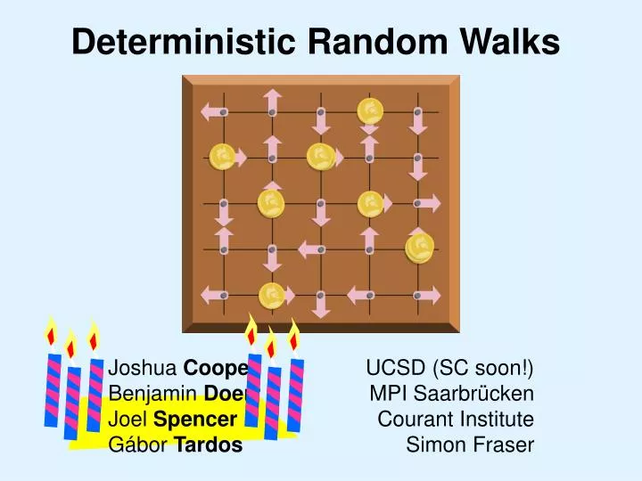
Deterministic Random Walks. Joshua Cooper Benjamin Doerr Joel Spencer Gábor Tardos. UCSD (SC soon!) MPI Saarbrücken Courant Institute Simon Fraser. t =1. t =2. t =3. An observation about cellular automata (see Wolfram’s NKS):. They generally fall into three categories.

E N D
Deterministic Random Walks Joshua Cooper Benjamin Doerr Joel Spencer Gábor Tardos UCSD (SC soon!) MPI Saarbrücken Courant Institute Simon Fraser
t =1 t =2 t =3 An observation about cellular automata (see Wolfram’s NKS): They generally fall into three categories.
An observation about cellular automata (see Wolfram’s NKS): They generally fall into three categories. I. Behavior so simple we can prove that a pattern emerges… II. Behavior so complicated you could simulate a Turing machine on it… III. And…
III. Behavior that is “randomlike”… Such automata are useful: 1. Fast pseudorandom number generation 2. Quasi-Monte Carlo integration 3. Bounds in discrepancy theory / quasirandomness However, very little is usually known outside of experimental results…
“The P-Machine” 1. At every step of (discrete) time, every chip moves. 2. When a single chip moves, it goes in the direction that its “rotor” is pointing. 3. When a chip moves, its rotor turns 90°.
9 1 10 t=0 1. At every step of (discrete) time, every chip moves. 2. When a single chip moves, it goes in the direction that its “rotor” is pointing. 3. When a chip moves, its rotor turns 90°.
1 8 1 9 t=0 1. At every step of (discrete) time, every chip moves. 2. When a single chip moves, it goes in the direction that its “rotor” is pointing. 3. When a chip moves, its rotor turns 90°.
1 7 1 8 1 t=0 1. At every step of (discrete) time, every chip moves. 2. When a single chip moves, it goes in the direction that its “rotor” is pointing. 3. When a chip moves, its rotor turns 90°.
1 6 1 7 1 1 t=0 1. At every step of (discrete) time, every chip moves. 2. When a single chip moves, it goes in the direction that its “rotor” is pointing. 3. When a chip moves, its rotor turns 90°.
1 1 5 2 6 1 1 t=0 1. At every step of (discrete) time, every chip moves. 2. When a single chip moves, it goes in the direction that its “rotor” is pointing. 3. When a chip moves, its rotor turns 90°.
2 1 4 2 5 1 1 t=0 1. At every step of (discrete) time, every chip moves. 2. When a single chip moves, it goes in the direction that its “rotor” is pointing. 3. When a chip moves, its rotor turns 90°.
2 1 3 2 4 2 1 t=0 1. At every step of (discrete) time, every chip moves. 2. When a single chip moves, it goes in the direction that its “rotor” is pointing. 3. When a chip moves, its rotor turns 90°.
2 1 2 2 3 2 2 t=0 1. At every step of (discrete) time, every chip moves. 2. When a single chip moves, it goes in the direction that its “rotor” is pointing. 3. When a chip moves, its rotor turns 90°.
2 2 1 3 2 2 2 t=0 1. At every step of (discrete) time, every chip moves. 2. When a single chip moves, it goes in the direction that its “rotor” is pointing. 3. When a chip moves, its rotor turns 90°.
3 2 3 1 2 2 t=0 1. At every step of (discrete) time, every chip moves. 2. When a single chip moves, it goes in the direction that its “rotor” is pointing. 3. When a chip moves, its rotor turns 90°.
3 2 3 2 t=1 1. At every step of (discrete) time, every chip moves. 2. When a single chip moves, it goes in the direction that its “rotor” is pointing. 3. When a chip moves, its rotor turns 90°.
+.5 2.5 -.5 +.5 2.5 10 2.5 -.5 2.5 Compare to the “linear machine” : splits chips evenly among neighbors. How large can the difference be? Same as the expected value for a simple random walk on the graph.
Theorem 1 (C., Spencer ’05). The difference at any point, after any amount of ✴ any initial configuration of rotors, time, with any initial configuration of chips, is bounded by a constant cd that depends only on and any rotor permutations, the dimension d. ✴ any even configuration. Remark. This is best possible in the senses that: a.) The statement is false for mixed even/odd configurations. b.) cd is a computable constant, with c1≈2.29. c.) The rotors can each go through a different permutation of the 2ddirections.
Amazingly, we can say something much stronger… Restrict our attention to d = 1, i.e., a P-machine on the integers: Definition. Write Δ(x,t) for the discrepancy between the P-machine and the linear machine at the point x at time t. Definition. Write Δ(S,Z) for the discrepancy on a set S over all times in Z, i.e.,
Theorem (C., Doerr, Tardos, Spencer) : L∞for Space-Intervals for intervals I of length L. Theorem (CDTS) : L2for Space-Intervals for intervals I of length L, and M sufficiently large. Corollary (CDTS) : For “most” translates of an interval,
Theorem (CDTS) : L∞for Time-Intervals for intervals J of length T. Theorem (CDTS) : L∞for Space-Time-Intervals for intervals I of length L and intervals J of length T.
Not only that… but ALL of these results are best possible. That is, there exist (different) initial configurations of chips and rotors so that, for any given intervals I, J with lengths L and T, respectively,
The upper bounds are proved by counting the contributions to the final quantity that each chip makes at each time. Lots of cancellation translates to small discrepancies. For the lower bounds, we show that all the arguments can be reversed, i.e., there is a sequence of chips-and-arrows so that the upper bound is achieved. Two crucial tools...
Theorem (CDST) : Parity-Forcing For any initial position of the arrows and any :ℤ×ℕ0→{0,1}, there exists an initial even configuration of the chips such that for all xℤ, tℕ0 such that x≡t(mod 2), we have chips(x,t)≡(x,t)(mod 2). This follows from the following statement… Theorem (CDST) : Arrow-Forcing Let ρ:ℤ×ℕ0→{left, right} be defined arbitrarily. There exists an even initial configuration that results in the arrows agreeing with ρ(x,t) for all xand t with x≡t(mod 2).
Conjecture: The probability that v is visited at time t in a random walk started from the origin, p(v, t), is unimodal (in t 2ℤ). For a function χ : ℤd → ℝ, define The proof would have been easier if only… Definition: p(v, t) is the probability that a chip leaving from 0 arrives at v at time t in a simple random walk Conjecture: p(χ, t)is the concatenation of a finite number of monotone subsequences, depending only on |supp(χ)|.
This set-up can be vastly generalized: Given a graph G, and functions f : V(G) → ℕ0the initial number of chips r : V(G) →V(G)* with r(v) a permutation of N(v)the rotor sequences Define chips(x,t) = chip count at x at time t for a P-machine on G. Define E(x,t) = chip count at x at time t for a linear machine on G.
Question: For which bipartite G must chips(x,t)-E(x,t) remain bounded for any x, t, r, and f with supp( f ) in one color class? Theorem (CDS’05): Not the infinite regular tree. Wild and Unfounded Guess: It has something to do with amenability. THANK YOU!