First Sky Demonstration of Potential for Ground Layer Adaptive Optics Correction

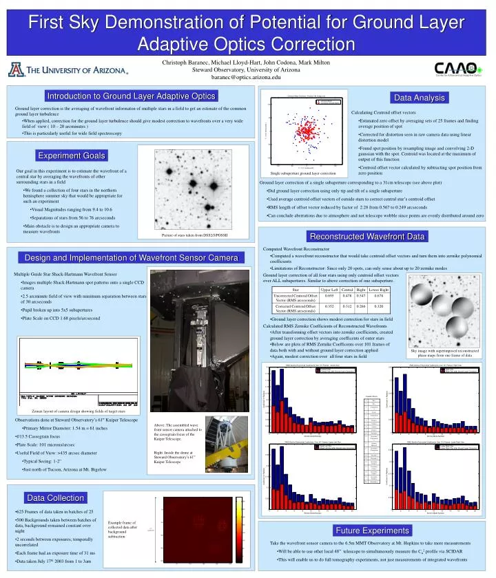
1. Center for Astronomical Adaptive Optics First Sky Demonstration of Potential for Ground Layer Adaptive Optics Correction Christoph Baranec, Michael Lloyd-Hart, John Codona, Mark Milton Steward Observatory, University of Arizona baranec@optics.arizona.edu Introduction to Ground Layer Adaptive Optics Data Analysis • Ground layer correction is the averaging of wavefront informaton of multiple stars in a field to get an estimate of the common ground layer turbulence • When applied, correction for the ground layer turbulence should give modest correction to wavefronts over a very wide field of view ( 10 – 20 arcminutes ) • This is particularly useful for wide field spectroscopy • Calculating Centroid offset vectors • Estimated zero offset by averaging sets of 25 frames and finding average position of spot • Corrected for distortion seen in raw camera data using linear distortion model • Found spot position by resampling image and convolving 2-D gaussian with the spot. Centroid was located at the maximum of output of this function • Centroid offset vector calculated by subtracting spot position from zero position Experiment Goals • Our goal in this experiment is to estimate the wavefront of a central star by averaging the wavefronts of other surrounding stars in a field • We found a collection of four stars in the northern hemisphere summer sky that would be appropriate for such an experiment • Visual Magnitudes ranging from 9.4 to 10.6 • Separations of stars from 56 to 76 arcseconds • Main obstacle is to design an appropriate camera to measure wavefronts Single subaperture ground layer correction • Ground layer correction of a single subaperture corresponding to a 31cm telescope (see above plot) • Did ground layer correction using only tip and tilt of a single subaperture • Used average centroid offset vectors of outside stars to correct central star’s centroid offset • RMS length of offset vector reduced by factor of 2.28 from 0.567 to 0.249 arcseconds • Can conclude aberrations due to atmosphere and not telescope wobble since points are evenly distributed around zero Reconstructed Wavefront Data Picture of stars taken from DSS2/J/POSSII • Computed Wavefront Reconstructor • Computed a wavefront reconstructor that would take centroid offset vectors and turn them into zernike polynomial coefficients • Limitations of Reconstructor: Since only 20 spots, can only sense about up to 20 zernike modes • Ground layer correction of all four stars using only centroid offset vectors • over ALL subapertures. Similar to above correction of one subaperture. • Ground layer correction shows modest correction for stars in field • Calculated RMS Zernike Coefficients of Reconstructed Wavefronts • After transforming offset vectors into zernike coefficients, created • ground layer correction by averaging coefficents of outer stars • Below are plots of RMS Zernike Coefficents over 101 frames of • data both with and without ground layer correction applied • Again, modest correction over all four stars in field Design and Implementation of Wavefront Sensor Camera • Multiple Guide Star Shack-Hartmann Wavefront Sensor • Images multiple Shack-Hartmann spot patterns onto a single CCD camera • 2.5 arcminute field of view with minimum separation between stars of 30 arcseconds • Pupil broken up into 5x5 subapertures • Plate Scale on CCD 1.68 pixels/arcsecond Sky image with superimposed reconstructed phase maps from one frame of data Zernike Modes Zemax layout of camera design showing fields of target stars • Observations done at Steward Observatory’s 61" Kuiper Telescope • Primary Mirror Diameter: 1.54 m = 61 inches • f/13.5 Cassegrain focus • Plate Scale: 101 microns/arcsec • Useful Field of View: >435 arcsec diameter • Typical Seeing: 1-2" • Just north of Tucson, Arizona at Mt. Bigelow Above: The assembled wave front sensor camera attached to the cassegrain focus of the Kuiper Telescope. Right: Inside the dome at Steward Observatory’s 61” Kuiper Telescope Data Collection • 625 Frames of data taken in batches of 25 • 500 Backgrounds taken between batches of data, background remained constant over night • 2 seconds between exposures; temporally uncorrelated • Each frame had an exposure time of 31 ms • Data taken July 17th 2003 from 1 to 3am Example frame of collected data after background subtraction Future Experiments 2.5 arcminutes • Take the wavefront sensor camera to the 6.5m MMT Observatory at Mt. Hopkins to take more measurements • Will be able to use other local 48” telescope to simultaneously measure the Cn2 profile via SCIDAR • This will enable us to do full tomography experiments, not just measurements of integrated wavefronts