Download
1 / 49
490 likes | 603 Views
Options. Chapter 28. Background. Put and call prices are affected by Price of underlying asset Option’s exercise price Length of time until expiration of option Volatility of underlying asset Risk-free interest rate Cash flows such as dividends

E N D
Options Chapter 28 Chapter 28: Options
Background • Put and call prices are affected by • Price of underlying asset • Option’s exercise price • Length of time until expiration of option • Volatility of underlying asset • Risk-free interest rate • Cash flows such as dividends • Premiums can be derived from the above factors • Investors’ expectations about the direction of the underlying asset’s price change does not impact the value of an option Chapter 28: Options
Introduction to Binomial Option Pricing • A simple valuation model is used to determine the price for a call option • Assumes only two possible rates of return over time period • The price could either rise or fall • For instance, if a stock’s price is currently $45.45 and it can change by either ±10% over the next period, the possible prices are • $45.45 x 1.10 = $50 • $45.45 x 0.90 = $40.91 • Ignores taxes, commissions and margin requirements • Assumes investor can gain immediate use of short sale funds • Assume no cash flows are paid Chapter 28: Options
One-Period Binomial Call Pricing Formula • Intrinsic ValueCall = MAX[0, {Stock Price – Exercise Price}] • If the an option has an exercise price of $40 and • The stock price was $50 upon expiration the option would be valued at • COPUp = MAX[0,$50 - $40] = $10 • The stock price was $40.91 upon expiration the option would be valued at • COPDown = MAX[0, $40.91 - $40] = $0.91 Chapter 28: Options
One-Period Binomial Call Pricing Formula • If we borrowed the money needed to purchase the optioned security at the risk-free rate • We would not need to invest any money to get started (AKA: self-financing portfolio) • If the stock price rose the ending value of the portfolio would be • VUp = Value of stock – (1+ risk-free)(amount borrowed) • If the stock price fell the ending value of the portfolio would be • VDown = Value of stock – (1+ risk-free)(amount borrowed) Chapter 28: Options
One-Period Binomial Call Pricing Formula • To find the option’s price you must find the values for the amount of stock and borrowed funds that will equate COPUp and COPDown to ValueUp and ValueDown or • MAX [0, Price0Up – exercise price] = COPUp = ValueUp = Up value of stock – (1+risk-free rate × amount borrowed) • MAX [0, Price0Down – exercise price] = COPDown = ValueDown = Down value of stock – (1+risk-free rate × amount borrowed) • Equations can be solved simultaneously to determine the hedge ratio Chapter 28: Options
One-Period Binomial Call Pricing Formula • The hedge ratio represents the number of shares of stock costing P0 financed by borrowing B* dollars • This will duplicate the expiration payoffs from a call option Chapter 28: Options
One-Period Binomial Call Pricing Formula • The initial price (COP0) of the call option is • Hedge ratio × P0 – B* = COP0 • Observations • P0 is a major determinant of a call option’s initial price • The probability of the price fluctuations do not impact COP0 • Model is risk-neutral • Call has the same value whether investor is risk-averse, risk-neutral or risk-seeking Chapter 28: Options
Multi-Period Binomial Call Pricing Formula • One-period model can be used to • Encompass multiple time periods • Value common stock, bonds, mortgages • What if stock currently priced at $45.45 could either rise or fall in value by 10% over each of the next two time periods Chapter 28: Options
Multi-Period Binomial Call Pricing Formula Chapter 28: Options
Multi-Period Binomial Call Pricing Formula • This concept can be extended to any number of time periods • Can add cash flow payments to the branches • When a large number of small time periods are involved, we obtain Pascal’s triangle Chapter 28: Options
Multi-Period Binomial Call Pricing Formula Resembles a normal probability distribution as n increases. Chapter 28: Options
Multi-Period Binomial Call Pricing Formula • Pascal’s triangle in tree form Chapter 28: Options
Black and Scholes Call Option Pricing Model • Black & Scholes (B&S) developed a formula to price call options • Assume normally distributed rates of return Chapter 28: Options
[ ] ( ) + + ln RFR 0.5VAR(r) d XP P = 0 x 0.5 σ d B&S Call Valuation Formula • Use a self-financing portfolio • COP0 = (P0h – B) • Assume a hedge ratio of N(x) • Borrowings equal XP[e(-RFR)d]N(y) • B&S equation • COP0 = P0 N(x)- XP[e(-RFR)d]N(y) • where Fraction of year until call expires Values of x and y have no intuitive meaning. Chapter 28: Options
B&S Call Valuation Formula • N(x) is a cumulative normal-density function of x • Gives the probability that a value less than x will occur in a normal probability distribution • To use the B&S model you need • Table of natural logarithms (or a calculator) • Table of cumulative normal distribution probabilities Chapter 28: Options
Example • Given the following information, calculate the value of the call • P0 = $60 • XP (strike or exercise price) = $50 • d (time to expiration) = 4 months or 1/3 of a year • Risk-free rate = 7% • Variance (returns) = 14.4% Chapter 28: Options
Example • Substituting the values for N(x) and N(y) into the COP0 equation • COP0 = $60(0.853) - $50(0.977)(0.796) = $51.18 - $38.89 = $12.29 Looking this value up in the table yields an N(x) of 0.853. Looking this value up in the table yields an N(y) of 0.796. Chapter 28: Options
The Hedge Ratio • Represents the fraction of a change in an option’s premium caused by a $1 change in the price of the underlying asset • AKA delta, neutral hedge ratio, elasticity, equivalence ratio • Calls have a hedge ratio between 0 and 1 • Hedgers would like a hedge ratio that will completely eliminate changes in their hedged portfolio • Is presented as N(x) in the B&S equation • If x has a value of 1.65, N(x) has a value of 0.9505 • Means that 95.05 shares of a stock should be sold short to establish a perfect hedge against 100 shares in an offsetting position Chapter 28: Options
Risk Statistics and Option Values • Investor normally estimates an asset’s standard deviation of returns and uses it as an input into the B&S model • However, can insert the call’s current price into the model and compute the implied volatility of the underlying asset • Risk statistics change over time Chapter 28: Options
Put-Call Parity Formula • Formula represents an arbitrage-free relationship between put and call prices on the same underlying asset • If the two options have identical strike prices and times to maturity • Consider the following: Values are the same whether the stock is in or out of the money when options expire—thus portfolio is perfectly hedged. Chapter 28: Options
Put-Call Parity Formula • This portfolio is worth the present value of the option’s exercise price or • XP (1+RFR)d under either outcome • The portfolio must also be worth • P + POP – COP • This leads to the Put-Call Parity equation • P + POP – COP = XP (1+RFR)d Chapter 28: Options
Pricing Put Options • We can use put-call parity to value a put after the value of a call on the same security has been determined • POP= COP + (XP (1+RFR)d)– P • Example: Calculate the price of a put option on a stock with a current price of $60, a strike price of $50, 4 months remaining until expiration, a risk-free rate of 7% and a variance of 14.4% with a call valued at $12.29 • POP = $12.29 + (50 (1.07)0.333)-$60 = $1.18 Chapter 28: Options
Checking Alignment of Put and Call Prices • When prices for both puts and calls on the same underlying stock are available • Put-call parity can be used to determine if the prices are properly aligned • If not, arbitrage profits can be earned Chapter 28: Options
Example • Given information • On 7/12/2000 KO’s stock was selling for $57 • Call options with a strike price of $60 and one month until expiration were selling for $1.625 • Puts were selling for $4.125 • 3-month T-bills were yielding 6% • Plugging data into the put-call parity equation • 4.125 1.625 + 60/1.060.0833 – 57 • 4.125 4.3344 • Either puts were under priced by 21¢ or calls were over priced by 21¢ • Ignores transaction costs Chapter 28: Options
The Effects of Cash Dividend Payments • Ex-dividend date • First trading day after the cash dividend is paid • Stock trades at a reduced price • Reduced by the amount of the cash dividend • Stockholders are no longer entitled to the dividend, therefore they should not pay for it • The ex-dividend stock price drop-off • Reduces value of call options • Increases value of put options Chapter 28: Options
The Effects of Cash Dividend Payments • Impacts the value of an American call option Price curve reflects the option’s price if it is not exercised and not expired (alive). If the option’s live value before ex-dividend > value ex dividend by more than dividend, call should be exercised before it trades ex-dividend to capture cash dividend (while embedded in stock’s price). On the ex-dividend date the stock price drops from Pd to Pe. Option prices usually do not drop by the same amount because the slope of the price curve < +1. Chapter 28: Options
The Effects of Cash Dividend Payments • The present value of the cash dividend payment should be considered in the B&S option pricing model • COPe = [P0 – Div/(1+RFR)]N(x) – XP[e(-RFR)d]N(y) • Example • P0 = $60 • XP (strike or exercise price) = $50 • d (time to expiration) = 4 months or 1/3 of a year • Risk-free rate = 7% • Variance (returns) = 14.4% • Expected cash dividend of $2 in one year • Present value of dividend = $2/1.07 = $1.869 • COPe = [60 – 1.869]0.853 –50[0.977]0.796 = $10.69 The addition of the cash dividend has lowered the call value by $1.60. Chapter 28: Options
Options Markets • Chicago Board Options Exchange (CBOE) • Founded in 1973 but is now the largest options exchange in world • American Stock Exchange • Second largest options exchange • Many options transactions are cleared through • Options Clearing Corporation (OCC) • International Securities Exchange (ISE) • Opened in 2000 • Electronic exchange • Competes with CBOE, AMEX, PHIX, PSE Chapter 28: Options
Synthetic Positions Can Be Created From Options • Buying a call and selling a put on the same security • Creates the same position as a buy-and-hold position in the security • AKA synthetic long position Chapter 28: Options
Example • Given information • Phelps’ stock is currently trading for $40 a share • You buy a six-month call with a $40 exercise price for a $5 cost • You write an 8-month put with an exercise price of $40 for $5 in premium income Chapter 28: Options
Example • Contrasting the actual and synthetic long positions If the call and put prices , the synthetic position the actual position. Put-call parity shows that the price of a put must be < the price of a similar call. Thus, to make the put price = call price, put had to have a longer time to expiration (8 months vs. 6 months). Chapter 28: Options
Synthetic Positions Can Be Created From Options • Some investors prefer a synthetic long position to an actual long position • Requires smaller initial investment • Creates more financial leverage • Owner of a synthetic long position does not collect cash dividends or coupon interest from underlying securities as they do not actually own those securities • Also, when options expire additional premiums must be paid to re-establish position Chapter 28: Options
Synthetic Short Position • Can create a synthetic short position by • Selling (writing) a call and simultaneously buying a put with a similar exercise price on the same underlying stock • Superior to an actual short position in the stock • The premium income from selling the call should be > premium paid to buy the put • Requires a smaller initial investment than an actual short sell • Does not have to pay cash dividends on the optioned stock • Disadvantages of a synthetic short position • After expiration of option more money would have to be spent to re-establish position • Could accumulate unlimited losses if the stock price rose high enough Chapter 28: Options
Writing Covered Calls • Covered call • Writing a call option against securities you already own • Cover the writer’s exposure to potential loss • If call owner exercises the option • Option-writer delivers the already owned securities without having to buy them in the market • Not all covered call positions are profitable • If stock price falls • Long position in underlying stock decreases • However, receive call premium income Chapter 28: Options
Writing Covered Calls • Naked call writing • Occurs when call writer does not own the underlying security • Risky if the price of the underlying security increases • Initial margin of 15% or more required • Whereas a covered option writer does not have to put up extra margin to write a covered call Chapter 28: Options
Writing Covered Calls • Covered call writers • Gain the most when stock price remains at exercise price and option expired unexercised • Receive premium income and get to keep the stock • If stock price increases significantly would have been better off not having written the option • Will have to give security to exerciser Chapter 28: Options
Straddles • Straddle occurs when • Equal number of puts and calls are bought on the same underlying asset • Must have same maturity and strike price • Long straddle position • Profit if optioned asset either • Experiences a large increase in price • Experiences a large decrease in price • Experiences large increases and decreases in price • Useful for a stock experiencing great deal of volatility Chapter 28: Options
Long Straddle Position • Infinite number of break-even points for a long straddle position • Downside limit • Sum of put and call prices • Upside limit • Sum of put and call prices • Believe the underlying stock has potential for enough price movements to make the straddle profitable before expiration • Only a small probability of losing the aggregate premium outlay Chapter 28: Options
Short Straddle Position • Symmetrically opposite to long straddle position • Believe stock price will not vary significantly before options expire • Probability that straddle will keep 100% of premium income is small Chapter 28: Options
Spreads • The purchase of one option and sale of a similar but different option • Can be either puts or calls but not puts and calls • Spread can occur based on • Different strike prices (vertical spreads) • Different expirations (horizontal spreads) • Time spreads, calendar spreads Chapter 28: Options
Spreads • Diagonal spreads combine vertical and horizontal spreads • Credit spreads • Generate premium income exceeding related costs • Debit spreads • Generate an initial cash outflow Chapter 28: Options
Strangles • Involves a put and call with same expiration date but different strike prices • Involves smaller total outlay than a straddle Chapter 28: Options
Strangles • Long strangle • Debit transaction • No premiums from writing options are received • Short strangle • Credit transaction • No outlays • Small premiums received but also small chance options will be exercised against writer Chapter 28: Options
Bull Spread • Vertical spread involving two calls with same expiration date • Debit transaction • Used if believe price of underlying asset will rise, but not significantly Chapter 28: Options
Bear Spread • Vertical spread involving two puts with same expiration date but different strike prices • Are profitable only if asset price declines between the two exercise prices • Losses are limited if expectations are incorrect Chapter 28: Options
Butterfly Spreads • Combination of a bull and bear spread on the same underlying security • Long butterfly spread • Will maximize profit if underlying asset’s price does not fluctuate from XPB • Short butterfly spread • Profitable if optioned asset experiences large up and/or down price fluctuations Chapter 28: Options
The Bottom Line • Binomial option pricing model • Mathematically simple • B&S Option Pricing Model • First closed-form option pricing model • Binomial option pricing model is equivalent to B&S if there are an infinite number of tiny time periods • Put prices can be determined using put-call parity formula Chapter 28: Options
The Bottom Line • Ex-dividend stock price drop-off decreases (increases) value of a call (put) option • Puts and calls can be assembled to build more complex investing positions • Can build a position that will allow investor to benefit if price of underlying asset • Rises • Falls • Fluctuates up and down • Never changes • Options allow us to analyze securities in ways we might not have originally realized Chapter 28: Options