Download
1 / 10
270 likes | 775 Views
Model Predictive Control (MPC). rev. 2.8 of May 25, 2018 by M. Miccio. Introduction on MPC. Introduced since 1980 It works in discrete time framework It partly overcomes the need of a feedback architecture

E N D
Model Predictive Control (MPC) rev. 2.8 of May 25, 2018 by M. Miccio from Seborg, Edgar, Mellichamp, Process Dynamics and Control, 2nd Ed
Introduction on MPC • Introduced since 1980 • It works in discrete time framework • It partly overcomes the need of a feedback architecture • It better handles complicate dynamics (large dead time, inverse response, etc.) present in a wide system • It integrates dynamic modeling and optimization • It is inherently multi-variable • It may integrate feedforward control • It does more thanset pointtrackingand disturbancerejection … from Seborg, Edgar, Mellichamp, Process Dynamics and Control, 2nd Ed
Side Objectives of Model Predictive Control • Prevent violations of constraints on input (manipulated) and output (controlled) variables. • Prevent excessive movement of the input (manipulated) variables. • Drive some output (controlled) variables to their optimal set points, while maintaining other outputs within specified ranges. • If a sensor or actuator becomes not available anymore, still control as much of the process as possible. from Seborg, Edgar, Mellichamp, Process Dynamics and Control, 2nd Ed
Model Predictive Control: Conceptual schematics from ControlWiki
Model Predictive Control: schematics of time evolution y* y* reference trajectory Manipulated variable Figure 20.2 Basic concept for Model Predictive Control from Seborg, Edgar, Mellichamp, Process Dynamics and Control, 2nd Ed
Model Predictive Control: Calculations modules • The reference trajectory y*(k) is obtained, based on set points calculated using Real Time Optimization (RTO). • Future values of state/output variables ŷ(•) are predicted using a dynamic model of the process and current measurements at the k-th sampling instant, for a given sequence of future control inputs u(k). ŷ(k+1)=f [ŷ(k), u(k)] • Unlike time delay compensation methods, the predictions are made for more than one time delay ahead until the prediction horizon P ( N) • Inequality & equality constraints, and measured disturbances are included in the model calculations. • The manipulated variablesu(•) are calculated at the k-th sampling instant for a future time length set as M ( N), i.e., the control horizon,so that they minimize a given objective function J. For example: • Typically, an LP or QP problem is solved from Seborg, Edgar, Mellichamp, Process Dynamics and Control, 2nd Ed
Model Predictive Control: Calculation sequence • At the k-th sampling instant • The set of M“control moves”, i.e.,the values of the manipulated variablesu at the next M sampling instants, {u(k), u(k+1), …, u(k+M -1)} are calculated so as to minimize the predicted deviations from the reference trajectory over the next P sampling instants while satisfying the constraints. • Terminology: M = control horizon, P = prediction horizon • Then, the first “control move”u(k) is implemented in plant control until the next sampling instant k+1 • At the next sampling instant, k+1, • the M-step control policy is re-calculated for the next M sampling instants, k+1 to k+M, and the first control move u(k+1) is implemented. • Then, steps are repeated for subsequent sampling instants. This is an example of a receding horizon approach. Although a sequence of M control moves is calculated at each sampling instant, only the first move is actually implemented from Seborg, Edgar, Mellichamp, Process Dynamics and Control, 2nd Ed
Model Predictive Control MPC is like … … playing chess and planning moves ahead
Real-Time Optimization (RTO) • The on-line calculation of optimal set-points, also called real-time optimization (RTO), allows the profits from the process to be maximized while satisfying operating constrains imposed on some relevant process variables. • In real-time optimization (RTO), the optimum values of the set points are re-calculated on a regular basis (e.g., every hour or every day). • These repetitive calculations involve solving a constrained, economic optimization problem, based on: • A steady-state model of the process, traditionally a linear one • Economic information (e.g., prices, costs) • A performance Index to be maximized (e.g., profit) or minimized (e.g., cost). Note: Items # 2 and 3 are sometimes referred to as an economic model. Chapter 19
When Should Predictive Control be Used? MPC displays its main strength when applied to problems with • Processes are difficult to control with standard PID algorithm (e.g., large time constants, substantial dead times, inverse response, etc.) • There is a large number of manipulated (u) and controlled variables (y) • There is significant process interactions between u and y • i.e., more than one manipulated variable has a significant effect on an important process variable. • Constraints (limits) on process variables and manipulated variables are important for normal control • There are multiple disturbances; if they can be measured, this exploits the built-in feedforward capabilities of MPC from Seborg, Edgar, Mellichamp, Process Dynamics and Control, 2nd Ed