RAID & Performance: Exploring Disk Arrays and Flash Memory

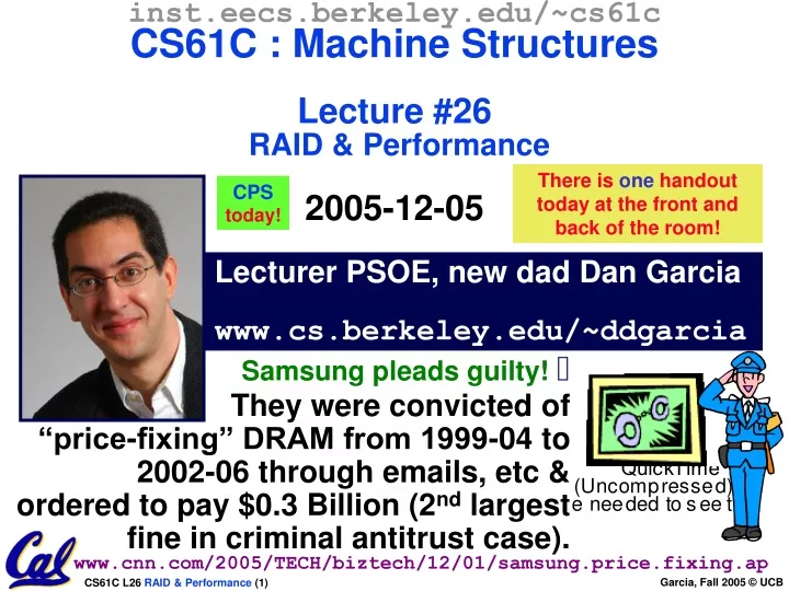
1. inst.eecs.berkeley.edu/~cs61cCS61C : Machine StructuresLecture #26RAID & Performance2005-12-05 There is one handout today at the front and back of the room! CPStoday! Lecturer PSOE, new dad Dan Garcia www.cs.berkeley.edu/~ddgarcia Samsung pleads guilty!They were convicted of“price-fixing” DRAM from 1999-04 to 2002-06 through emails, etc &ordered to pay $0.3 Billion (2nd largest fine in criminal antitrust case). www.cnn.com/2005/TECH/biztech/12/01/samsung.price.fixing.ap

2. 1 inch disk drive! • 2005 Hitachi Microdrive: • 40 x 30 x 5 mm, 13g • 8 GB, 3600 RPM, 1 disk, 10 MB/s, 12 ms seek • 400G operational shock, 2000G non-operational • Can detect a fall in 4” andretract heads to safety • For iPods, cameras, phones • 2006 MicroDrive? • 16 GB, 12 MB/s! • Assuming past trends continue www.hitachigst.com

3. Where does Flash memory come in? • Microdrives and Flash memory (e.g., CompactFlash) are going head-to-head • Both non-volatile (no power, data ok) • Flash benefits: durable & lower power(no moving parts) • Flash limitations: finite number of write cycles (wear on the insulating oxide layer around the charge storage mechanism) • OEMs work around by spreading writes out • How does Flash memory work? • NMOS transistor with an additional conductor between gate and source/drain which “traps” electrons. The presence/absence is a 1 or 0. • wikipedia.org/wiki/Flash_memory

4. What does Apple put in its iPods? Thanks to Andy Dahl for the tip shuffle nano mini iPod Toshiba 1.8-inch 30,60GB(MK1504GAL) Toshiba 0.5,1GBflash Samsung 2,4GBflash Hitachi 1 inch 4,6GBMicroDrive

5. Use Arrays of Small Disks… • Katz and Patterson asked in 1987: • Can smaller disks be used to close gap in performance between disks and CPUs? Conventional: 4 disk designs 3.5” 5.25” 10” 14” High End Low End Disk Array: 1 disk design 3.5”

6. Replace Small Number of Large Disks with Large Number of Small Disks! (1988 Disks) IBM 3390K 20 GBytes 97 cu. ft. 3 KW 15 MB/s 600 I/Os/s 250 KHrs $250K x70 23 GBytes 11 cu. ft. 1 KW 120 MB/s 3900 IOs/s ??? Hrs $150K IBM 3.5" 0061 320 MBytes 0.1 cu. ft. 11 W 1.5 MB/s 55 I/Os/s 50 KHrs $2K Capacity Volume Power Data Rate I/O Rate MTTF Cost 9X 3X 8X 6X Disk Arrays potentially high performance, high MB per cu. ft., high MB per KW, but what about reliability?

7. Array Reliability • Reliability - whether or not a component has failed • measured as Mean Time To Failure (MTTF) • Reliability of N disks = Reliability of 1 Disk ÷ N(assuming failures independent) • 50,000 Hours ÷ 70 disks = 700 hour • Disk system MTTF: Drops from 6 years to 1 month! • Disk arrays too unreliable to be useful!

8. Review • Magnetic disks continue rapid advance: 2x/yr capacity, 2x/2-yr bandwidth, slow on seek, rotation improvements, MB/$ 2x/yr! • Designs to fit high volume form factor • RAID • Motivation: In the 1980s, there were 2 classes of drives: expensive, big for enterprises and small for PCs. They thought “make one big out of many small!” • Higher performance with more disk arms per $ • Adds option for small # of extra disks (the “R”) • Started @ Cal by CS Profs Katz & Patterson

9. Redundant Arrays of (Inexpensive) Disks • Files are “striped” across multiple disks • Redundancy yields high data availability • Availability: service still provided to user, even if some components failed • Disks will still fail • Contents reconstructed from data redundantly stored in the array  Capacity penalty to store redundant info  Bandwidth penalty to update redundant info

10. Berkeley History, RAID-I • RAID-I (1989) • Consisted of a Sun 4/280 workstation with 128 MB of DRAM, four dual-string SCSI controllers, 28 5.25-inch SCSI disks and specialized disk striping software • Today RAID is > $32 billion dollar industry, 80% nonPC disks sold in RAIDs

11. “RAID 0”: No redundancy = “AID” • Assume have 4 disks of data for this example, organized in blocks • Large accesses faster since transfer from several disks at once This and next 5 slides from RAID.edu, http://www.acnc.com/04_01_00.html

12. RAID 1: Mirror data •  Each disk is fully duplicated onto its “mirror” • Very high availability can be achieved • Bandwidth reduced on write: • 1 Logical write = 2 physical writes • Most expensive solution: 100% capacity overhead

13. RAID 3: Parity (RAID 2 has bit-level striping) • Parity computed across group to protect against hard disk failures, stored in P disk • Logically, a single high capacity, high transfer rate disk • 25% capacity cost for parity in this example vs. 100% for RAID 1 (5 disks vs. 8 disks)

14. RAID 4: parity plus small sized accesses • RAID 3 relies on parity disk to discover errors on Read • But every sector has an error detection field • Rely on error detection field to catch errors on read, not on the parity disk • Allows small independent reads to different disks simultaneously

15. Inspiration for RAID 5 • Small writes (write to one disk): • Option 1: read other data disks, create new sum and write to Parity Disk (access all disks) • Option 2: since P has old sum, compare old data to new data, add the difference to P: 1 logical write = 2 physical reads + 2 physical writes to 2 disks • Parity Disk is bottleneck for Small writes: Write to A0, B1 => both write to P disk A0 B0 C0 D0 P D1 P A1 B1 C1

16. RAID 5: Rotated Parity, faster small writes • Independent writes possible because of interleaved parity • Example: write to A0, B1 uses disks 0, 1, 4, 5, so can proceed in parallel • Still 1 small write = 4 physical disk accesses

17. RAID products: Software, Chips, Systems RAID was $32 B industry in 2002, 80% nonPC disks sold in RAIDs

18. Margin of Safety in CS&E? • Patterson reflects… • Operator removing good disk vs. bad disk • Temperature, vibration causing failure before repair • In retrospect, suggested RAID 5 for what we anticipated, but should have suggested RAID 6 (double failure OK) for unanticipated/safety margin…

19. Peer Instruction • RAID 1 (mirror) and 5 (rotated parity) help with performance and availability • RAID 1 has higher cost than RAID 5 • Small writes on RAID 5 are slowerthan on RAID 1 ABC 1: FFF 2: FFT 3: FTF 4: FTT 5: TFF 6: TFT 7: TTF 8: TTT

20. Administrivia • Please attend Wednesday’s lecture! • HKN Evaluations at the end • Compete in the Performance contest! • Deadline is Mon, 2005-12-12 @ 11:59pm,1 week from now • Sp04 Final exam + solutions online! • Final Review: 2005-12-11 @ 2pm in 10 Evans • Final: 2005-12-17 @ 12:30pm in 2050 VLSB • Only bring pen{,cil}s, two 8.5”x11” handwritten sheets + green. Leave backpacks, books, calculators, cells & pagers home!

21. Upcoming Calendar

22. Performance • Purchasing Perspective: given a collection of machines (or upgrade options), which has the • best performance ? • least cost ? • best performance / cost ? • Computer Designer Perspective: faced with design options, which has the • best performance improvement ? • least cost ? • best performance / cost ? • All require basis for comparison and metric for evaluation • Solid metrics lead to solid progress!

23. Plane DC to Paris TopSpeed Passen-gers Throughput (pmph) Boeing 747 6.5 hours 610 mph 470 286,700 BAD/Sud Concorde 3 hours 1350 mph 132 178,200 Two Notions of “Performance” • Which has higher performance? • Time to deliver 1 passenger? • Time to deliver 400 passengers? • In a computer, time for 1 job calledResponse Time or Execution Time • In a computer, jobs per day calledThroughput or Bandwidth

24. performance(x) = 1 execution_time(x) Definitions • Performance is in units of things per sec • bigger is better • If we are primarily concerned with response time " F(ast) is n times faster thanS(low)" means… performance(F)execution_time(S) n = = performance(S)execution_time(F)

25. Example of Response Time v. Throughput • Time of Concorde vs. Boeing 747? • Concord is 6.5 hours / 3 hours = 2.2 times faster • Throughput of Boeing vs. Concorde? • Boeing 747: 286,700 pmph / 178,200 pmph = 1.6 times faster • Boeing is 1.6 times (“60%”) faster in terms of throughput • Concord is 2.2 times (“120%”) faster in terms of flying time (response time) • We will focus primarily on execution time for a single job

26. Confusing Wording on Performance • Will (try to) stick to “n times faster”; its less confusing than “m % faster” • As faster means both increased performance and decreased execution time, to reduce confusion we will (and you should) use “improve performance” or “improve execution time”

27. What is Time? • Straightforward definition of time: • Total time to complete a task, including disk accesses, memory accesses, I/O activities, operating system overhead, ... • “real time”, “response time” or “elapsed time” • Alternative: just time processor (CPU) is working only on your program (since multiple processes running at same time) • “CPU execution time” or “CPU time” • Often divided intosystem CPU time (in OS)anduser CPU time (in user program)

28. How to Measure Time? • User Time  seconds • CPU Time: Computers constructed using a clock that runs at a constant rate and determines when events take place in the hardware • These discrete time intervals called clock cycles (or informally clocks or cycles) • Length of clock period: clock cycle time(e.g., 2 nanoseconds or 2 ns) and clock rate (e.g., 500 megahertz, or 500 MHz), which is the inverse of the clock period; use these!

29. Measuring Time using Clock Cycles (1/2) • or =Clock Cycles for a program Clock Rate • CPU execution time for a program =Clock Cycles for a program x Clock Cycle Time

30. Measuring Time using Clock Cycles (2/2) • One way to define clock cycles: Clock Cycles for program = Instructions for a program (called “Instruction Count”) x Average Clock cycles Per Instruction (abbreviated “CPI”) • CPI one way to compare two machines with same instruction set, since Instruction Count would be the same

31. Performance Calculation (1/2) • CPU execution time for program =Clock Cycles for program x Clock Cycle Time • Substituting for clock cycles: CPU execution time for program=(Instruction Count x CPI) x Clock Cycle Time =Instruction Count x CPIx Clock Cycle Time

32. CPU time = Instructions x Cycles x Seconds Program Instruction Cycle CPU time = Instructions x Cycles x Seconds Program Instruction Cycle CPU time = Instructions x Cycles x Seconds Program Instruction Cycle CPU time = Seconds Program Performance Calculation (2/2) • Product of all 3 terms: if missing a term, can’t predict time, the real measure of performance

33. CPI: • Calculate: Execution Time / Clock cycle time Instruction Count • Hardware counter in special register (PII,III,4) How Calculate the 3 Components? • Clock Cycle Time: in specification of computer (Clock Rate in advertisements) • Instruction Count: • Count instructions in loop of small program • Use simulator to count instructions • Hardware counter in spec. register • (Pentium II,III,4)

34. Calculating CPI Another Way • First calculate CPI for each individual instruction (add, sub, and, etc.) • Next calculate frequency of each individual instruction • Finally multiply these two for each instruction and add them up to get final CPI (the weighted sum)

35. Instruction Mix (Where time spent) Example (RISC processor) Op Freqi CPIi Prod (% Time) ALU 50% 1 .5 (23%) Load 20% 5 1.0 (45%) Store 10% 3 .3 (14%) Branch 20% 2 .4 (18%) 2.2 • What if Branch instructions twice as fast?

36. CPU time = Instructions x Cycles x Seconds Program Instruction Cycle “And in conclusion…” • RAID • Motivation: In the 1980s, there were 2 classes of drives: expensive, big for enterprises and small for PCs. They thought “make one big out of many small!” • Higher performance with more disk arms/$, adds option for small # of extra disks (the R) • Started @ Cal by CS Profs Katz & Patterson • Latency v. Throughput • Performance doesn’t depend on any single factor: need Instruction Count, Clocks Per Instruction (CPI) and Clock Rate to get valid estimations • User Time: time user waits for program to execute: depends heavily on how OS switches between tasks • CPU Time: time spent executing a single program: depends solely on processor design (datapath, pipelining effectiveness, caches, etc.)