Download
1 / 9
100 likes | 147 Views
• Objectives: Chernoff Bound Bhattacharyya Bound ROC Curves Discrete Features Resources: V.V. – Chernoff Bound J.G. – Bhattacharyya T.T. – ROC Curves NIST – DET Curves AAAS - Verification. ECE 8443 – Pattern Recognition. LECTURE 09: ERROR BOUNDS / DISCRETE FEATURES.

E N D
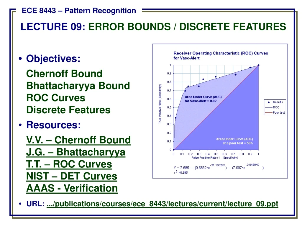
• Objectives: Chernoff Bound Bhattacharyya Bound ROC Curves Discrete Features Resources: V.V. – Chernoff Bound J.G. – Bhattacharyya T.T. – ROC Curves NIST – DET Curves AAAS - Verification ECE 8443 – Pattern Recognition LECTURE 09: ERROR BOUNDS / DISCRETE FEATURES • URL: .../publications/courses/ece_8443/lectures/current/lecture_09.ppt
09: ERROR BOUNDS MOTIVATION • Bayes decision rule guarantees lowest average error rate • Closed-form solution for two-class Gaussian distributions • Full calculation for high dimensional space difficult • Bounds provide a way to get insight into a problem and engineer better solutions. • Need the following inequality: Assume a b without loss of generality: min[a,b] = b. Also, ab(1- ) = (a/b)b and (a/b) 1. Therefore, b (a/b)b, which implies min[a,b] ab(1- ) . • Apply to our standard expression for P(error).
09: ERROR BOUNDS CHERNOFF BOUND • Recall: • Note that this integral is over the entire feature space, not the decision regions (which makes it simpler). • If the conditional probabilities are normal, this expression can be simplified.
where: 09: ERROR BOUNDS CHERNOFF BOUND FOR NORMAL DENSITIES • If the conditional probabilities are normal, our bound can be evaluated analytically: • Procedure: find the value of that minimizes exp(-k( ), and then compute P(error) using the bound. • Benefit: one-dimensional optimization using
where: 09: ERROR BOUNDS BHATTACHARYYA BOUND • The Chernoff bound is loose for extreme values • The Bhattacharyya bound can be derived by = 0.5: • These bounds can still be used if the distributions are not Gaussian (why? hint: maximum entropy). However, they might not be adequately tight.
09: ERROR BOUNDS RECEIVER OPERATING CHARACTERISITC • How do we compare two decision rules if they require different thresholds for optimum performance? • Consider four probabilities:
One system can be considered superior to another only if its ROC curve lies above the competing system for the operating region of interest. 09: ERROR BOUNDS GENERAL ROC CURVES • An ROC curve is typically monotonic but not symmetric:
where 09:DISCRETE FEATURES INTEGRALS BECOME SUMS • For problems where features are discrete: • Bayes formula involves probabilities (not densities): • Bayes rule remains the same: • The maximum entropy distribution is a uniform distribution: P(x=xi) = 1/N.
09: ERROR BOUNDS INTEGRALS BECOME SUMS • Consider independent binary features: • Assuming conditional independence: • The likelihood ratio is: • The discriminant function is: