Download
1 / 14
140 likes | 264 Views
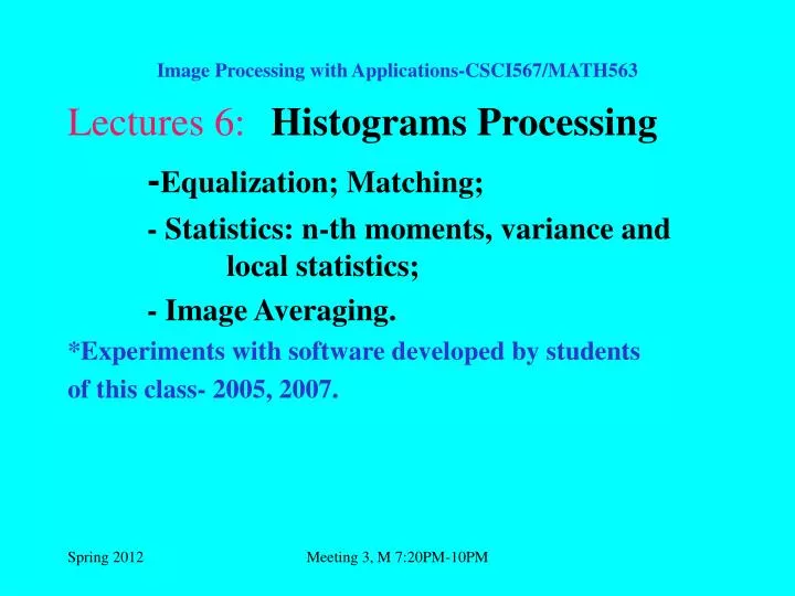
Image Processing with Applications-CSCI567/MATH563. Lectures 6: Histograms Processing - Equalization; Matching; - Statistics: n-th moments, variance and local statistics; - Image Averaging. *Experiments with software developed by students of this class- 2005, 2007.

E N D
Image Processing with Applications-CSCI567/MATH563 Lectures 6:Histograms Processing -Equalization; Matching; - Statistics: n-th moments, variance and local statistics; - Image Averaging. *Experiments with software developed by students of this class- 2005, 2007. Meeting 3, M 7:20PM-10PM
Histograms Processing Figure 1.a) An MRI image – brain section; b) The histogram of the image. Meeting 3, M 7:20PM-10PM
Histograms Matching Algorithm • Digital Image Processing, 3rd E, by Gonzalez, Woods Meeting 3, M 7:20PM-10PM
Exp. Results Histogram Matching and Equalization b) a) d) c) Figure 2. a) The original image; b) histogram; c) the image from (a)after matching with the histogram from b); d) the image from (a) after equalization. Experiments performed with a software coded by Nilkantha Aryal in a team with Sharon Rushing-2005. Meeting 3, M 7:20PM-10PM
Histograms Processing a) b) Figure 3. a) Images and their histograms; b) Central column histogram Equalized Images; right Column shows their Histograms. One could tell that images with good contrast have normal distribution of the gray levels. (Digital Image Processing, 2nd E, by Gonzalez, Woods). Meeting 3, M 7:20PM-10PM
Histograms Processing Figure 4. left) An image with a bad contrast; right) its histogram where most of the gray levels are distributed at the dark zone of the histogram.(Digital Image Processing, 2nd E, by Gonzalez, Richard). Meeting 3, M 7:20PM-10PM
Histograms Processing • b) • c) Figure 5. a) the curve used for histogram equalization; b) the image from Fig.4 after equalization; c) its histogram. (Digital Image Processing, 2nd E, by Gonzalez, Richard). Meeting 3, M 7:20PM-10PM
Histograms Processing Figure 6. Image enhancement using histograms matching. Meeting 3, M 7:20PM-10PM
Image Enhancement by Local Statistics Figure 7: (left) An image with low contrast right side. (right) The enhanced image by a local statistic image studio coded in C sharp, Spring 2007, by Josh D. Anderton, In a joint project with Renee Townsend. The original image is a courtesy of Digital Image Processing, 2nd E, by Gonzalez, Richard Meeting 3, M 7:20PM-10PM
Image Enhancement by Local Statistics-continuation of Lecture 3 Figure 8: (left) An X-ray image of a chest. (right) The enhanced image by a local statistic image studio coded in C sharp, Spring 2007, by Josh D. Anderton, In a joint project with Renee Townsend. Meeting 3, M 7:20PM-10PM
Image Planes Figure 9. a) the original image; b) - i) planes 1 to 8. Courtesy of Digital Image Processing, 2nd E, by Gonzalez, Richard Meeting 3, M 7:20PM-10PM
Arithmetic Logic Operations Figure 10. a) upper left-the original image; b) The lower 4 bits are set 0; c) Subtraction of the new image from the original; d) Equalized image from c). (Courtesy of Digital Image Processing, 2nd E, by Gonzalez, Richard). Meeting 3, M 7:20PM-10PM
Image Averaging • b) • d) • e) f) Figure 11. a) The original image; b) the image from (a) with added Gaussian noise: Mean=0, and deviation 64 gray level; c)-f) results averaging K=8,16,64,128. (Digital Image Processing, 2nd E, by Gonzalez, Richard). Meeting 3, M 7:20PM-10PM
Image Averaging Figure 12. a)-d) The result of subtracting the images given in Fig.11c)-f) from the image in 10a). Histograms of the result images. (Digital Image Processing, 2nd E, by Gonzalez, Richard). a) b) c) d) Meeting 3, M 7:20PM-10PM