Download
1 / 4
40 likes | 42 Views
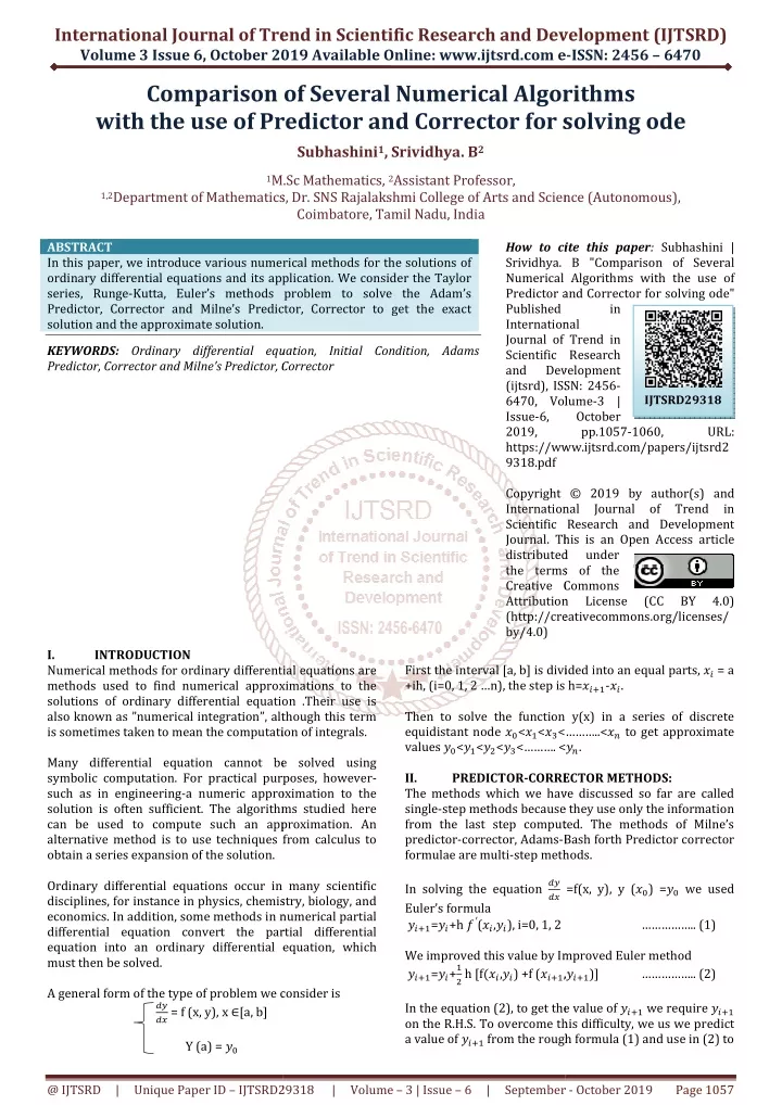
In this paper, we introduce various numerical methods for the solutions of ordinary differential equations and its application. We consider the Taylor series, Runge Kutta, Euler's methods problem to solve the Adam's Predictor, Corrector and Milne's Predictor, Corrector to get the exact solution and the approximate solution. Subhashini | Srividhya. B "Comparison of Several Numerical Algorithms with the use of Predictor and Corrector for solving ode" Published in International Journal of Trend in Scientific Research and Development (ijtsrd), ISSN: 2456-6470, Volume-3 | Issue-6 , October 2019, URL: https://www.ijtsrd.com/papers/ijtsrd29318.pdf Paper URL: https://www.ijtsrd.com/mathemetics/other/29318/comparison-of-several-numerical-algorithms-with-the-use-of-predictor-and-corrector-for-solving-ode/subhashini<br>

E N D
International Journal of Trend in Scientific Research and Development (IJTSRD) Volume 3 Issue 6, October 2019 2019 Available Online: www.ijtsrd.com e International Journal of Trend in Scientific Research and Development (IJTSRD) International Journal of Trend in Scientific Research and Development (IJTSRD) e-ISSN: 2456 – 6470 Comparison with the use of Predictor of Several Numerical Algorithms f Predictor and Corrector for solving Subhashini1, Srividhya. B2 of Several Numerical Algorithms or solving ode 1M.Sc Mathematics, M.Sc Mathematics, 2Assistant Professor, Mathematics, Dr. SNS Rajalakshmi College of Arts and Science Coimbatore, Tamil Nadu, India 1,2Department of Mathematics, nd Science (Autonomous), ABSTRACT In this paper, we introduce various numerical methods for the solutions of ordinary differential equations and its application. We consider the Taylor series, Runge-Kutta, Euler’s methods problem to solve the Adam’s Predictor, Corrector and Milne’s Predictor, Corrector to get the exact solution and the approximate solution. KEYWORDS: Ordinary differential equation, Initial Condition, Adams Predictor, Corrector and Milne’s Predictor, Corrector How to cite this paper Srividhya. B "Comparison of Several Numerical Algorithms with the use of Predictor and Corrector for solving ode" Published in International Journal of Trend in Scientific Research and Development (ijtsrd), ISSN: 2456 6470, Volume Issue-6, 2019, pp.1057 https://www.ijtsrd.com/papers/ijtsrd2 9318.pdf Copyright © 2019 by author(s) and International Journal of Trend in Scientific Research and Development Journal. This is an Open Access article distributed under the terms of the Creative Commons Attribution License (http://creativecommons.org/licenses/ by/4.0) How to cite this paper: Subhashini | Srividhya. B "Comparison of Several Numerical Algorithms with the use of Predictor and Corrector for solving ode" Published in International Journal of Trend in Scientific Research and Development (ijtsrd), ISSN: 2456- 6470, Volume-3 | October 2019, pp.1057-1060, https://www.ijtsrd.com/papers/ijtsrd2 In this paper, we introduce various numerical methods for the solutions of ordinary differential equations and its application. We consider the Taylor methods problem to solve the Adam’s Predictor, Corrector and Milne’s Predictor, Corrector to get the exact Ordinary differential equation, Initial Condition, Adams Predictor, Corrector IJTSRD29318 URL: Copyright © 2019 by author(s) and International Journal of Trend in ntific Research and Development Journal. This is an Open Access article distributed under the terms of the Creative Commons Attribution License http://creativecommons.org/licenses/ (CC (CC BY BY 4.0) 4.0) INTRODUCTION Numerical methods for ordinary differential equations are methods used to find numerical approximations to the solutions of ordinary differential equation .Their use is also known as ”numerical integration”, although this term I. Numerical methods for ordinary differential equations are methods used to find numerical approximations to the solutions of ordinary differential equation .Their use is also known as ”numerical integration”, although this term is sometimes taken to mean the computation of integrals. Many differential equation cannot be solved using symbolic computation. For practical purposes, however such as in engineering-a numeric approximation to the solution is often sufficient. The algorithms studied here can be used to compute such an approximation. An alternative method is to use techniques from calculus to obtain a series expansion of the solution. Ordinary differential equations occur in many scientific disciplines, for instance in physics, chemistry, biology, economics. In addition, some methods in numerical partial differential equation convert the partial differential equation into an ordinary differential equation, which must then be solved. A general form of the type of problem we consider is ?? ?? = f (x, y), x ∈[a, b] Y (a) = ?? First the interval [a, b] is divided into an equal parts, +ih, (i=0, 1, 2 …n), the step is h= Then to solve the function y(x) in a series of discrete equidistant node ??<??<??<………..< values ??<??<??<??<………. < II. PREDICTOR-CORRECTOR METHODS: The methods which we have discussed so far are called single-step methods because they use only the information from the last step computed. The methods of Milne’s predictor-corrector, Adams-Bash forth Predictor corrector formulae are multi-step methods. In solving the equation Euler’s formula ????=??+h ?′(??,??), i=0, 1, 2 We improved this value by Improved ????=??+? In the equation (2), to get the value of on the R.H.S. To overcome this difficulty, we us we predict a value of ???? from the rough formula (1) and use in (2) to from the rough formula (1) and use in (2) to First the interval [a, b] is divided into an equal parts, ?? = a +ih, (i=0, 1, 2 …n), the step is h=????-??. Then to solve the function y(x) in a series of discrete <………..<?? to get approximate <………. <??. e computation of integrals. Many differential equation cannot be solved using symbolic computation. For practical purposes, however- a numeric approximation to the solution is often sufficient. The algorithms studied here d to compute such an approximation. An alternative method is to use techniques from calculus to CORRECTOR METHODS: The methods which we have discussed so far are called step methods because they use only the information from the last step computed. The methods of Milne’s Bash forth Predictor corrector step methods. ?? ?? Ordinary differential equations occur in many scientific disciplines, for instance in physics, chemistry, biology, and economics. In addition, some methods in numerical partial differential equation convert the partial differential equation into an ordinary differential equation, which =f(x, y), y (??) =?? we used …………….. (1) We improved this value by Improved Euler method ? h [f???,??) +f (????, ,????)] …………….. (2) A general form of the type of problem we consider is In the equation (2), to get the value of ???? we require ???? To overcome this difficulty, we us we predict @ IJTSRD | Unique Paper ID – IJTSRD293 29318 | Volume – 3 | Issue – 6 | September 6 | September - October 2019 Page 1057
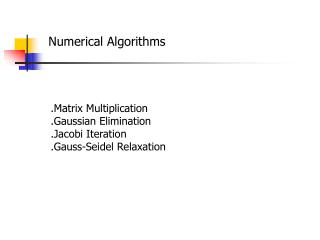
International Journal of Trend in Scientific Research and Development (IJTSRD) @ www.ijtsrd.com eISSN: 2456-6470 correct the value. Every time, we improve using (2). Hence equation (1) Euler’s formula is a predictor and (2) is a corrector. A predictor formula is used to predict the value of y at ???? and a corrector formula is used to corrector the error and to improve that value of????. 2.1.Milne’s Predictor Corrector Formula The Milne-Simpson method is a Predictor method. It uses a Milne formula as a Predictor and the popular Simpson’s formula as a Corrector. These formulae are based on the fundamental theorem of calculus. Y (????) = y (??) + ? ???,?) ?? When j=i-3, the equation .becomes an open integration formula and produces the Milne’s formulae ????,?=????+ ?? Similarly, When j=i-1, equation becomes a closed form integration and produces the two-segment Simpson’s formula ???? ,?=???? +? Milne’s formula is used to ‘predict’ the value of ????which is then used to calculate ???? ????=??????, ????) Then, equation (6) is used to correct the predicted value of????. The Process for the next value of i.Each stage involves four basic calculations,namely, 1.Prediction of ???? 2.evaluation of???? 3.correction of???? 4.improved value of ????(for use in next stage ) It is also possible to use the corrector formula repeatedly to refine the estimate of ???? before moving on the next stage. 2.2.Adams-Bash forth-Moulton Method Another popular fourth-order predictor-corrector method is the Adams-Bash forth-Moulton Method multistep method. The predictor formula is known as Adams- Bash forth predictor and is given by ???? = ??+? The corrector formula is known as Adams-Moulton Corrector and is given by ???? = ??+? This pair of equations can be implemented using the procedure described for Milne-Simpson ???ℎ??. TAYLOR SERIES METHOD In mathematics, a Taylor Series is a representation of a function as an infinite sum of terms that are calculated from the values of the functions derivatives at a single point The numerical solution of the equation ?? EULER’S METHOD Euler’s method is the simplest one-step method and has a limited application because of its low accuracy. However, it is discussed here as it serves as a starting point for all other advanced methods. Given the differential equation ?? ??=f(x, y) Given the initial condition y (??) = ?? We have ?? And therefore Y(x) =y (??)+ (x -??) ????, ??) Then the value of y(x) at x=?? is given by Y (??) = y (??)+ (?? –??) ????, ?? Letting h=?? -??, we obtain ??=??+h????, ??) Similarly, y(x) at x=?? is given by ??=??+h????, ?? ) In general, we obtain a recursive relation as ????=??+h????, ?? ); n= 0, 1, 2…………… Improved Euler method Let the tangent at???, ??) to the curve be ??A. In the interval???, ??), by previous approximate the curve by the tangent ??A. ????)=??+h????, ?? ) Where ????)=???? ??( ??, ????)). Let ?? C be line at ?? whose slope is f ( ??, ????)). Now take the average of the slopes at ?? and ?? i.e. ? ?[????, ?? )+f ( ??, ????))] Now draw line ??D through ?????, ?? ) with this as the slope. That is, y-??= ? This line intersects x=?? at ??=??+ ? ??=??+ ? Writing generally, ????=??+ ? RUNGE-KUTTA METHODS Runge-Kutta method reduces data requirements to reach the same precision without higher derivative calculation. The numerical solutions of the numerical equation ?? Given the initial condition y ???) = ??the fourth order Runge-Kutta method algorithm is mostly used in problems unless otherwise mentioned. ??=ℎ ???, ?) ??=ℎ ??? + ???? dx ………….. (3) ??=????, ??) ?(2????-????+2??) ………….. (4) ? (????+4??+????) ………….. (5) is then repeated Euler’s method, we ?[????, ??) +f ( ??, ????))] (x-??) ?? (55??-59????+37????-9????) ………….. (6) ?ℎ[????, ??) +f ( ??, ????))] ?ℎ[????, ??) + ????, ??+h ????, ??))] ?? (????-5??+19????-9????) ………….. (7) ?ℎ[????, ??) + ????+ ℎ,??+h? ?? ?,? ?))] ??=f?x, y) ??=f(x, y) Given the initial condition y (??) = ?? ??=y (??)= ??+? ? ?ℎ, ? + ? ???) ?!??′+?? ?!??′′+………………… @ IJTSRD | Unique Paper ID – IJTSRD29318 | Volume – 3 | Issue – 6 | September - October 2019 Page 1058
International Journal of Trend in Scientific Research and Development (IJTSRD) @ www.ijtsrd.com eISSN: 2456-6470 ? ?ℎ, ? + ? ?ℎ, ? + ? ???) ? ???) Adam’s corrector formula ??,?=1.362+0.0042[17.4843+31.578-7.1+1.2] =1.5433 3. Determine the value of y (0.4) using Milne’s method given ??=x+y, y (0) =1 use Improved Euler’s method to get the values of y (0.1), y (0.2) and y (0.3). ??=ℎ ??? + ??=ℎ ??? + ∆?=? EXAMPLE 1. Determine the value of y (0.4) using Milne’s method given ??=x+y, y (0) =1 use Taylor series to get the values of y (0.1), y (0.2) and y (0.3). Solution. Here ??=0, ??=1, ??=0.1, ??=0.2, ??=0.3, ??=0.4 ?′= ? + ???′=??+?? =0+1 =1 =y (0.4) ????+2??+2??+??) ????=??+ ? ?ℎ[????, ??) + ????+ ℎ,??+h ????, ??)] ??=1+ ? =1.11 ?(0.1) [?(0, 1) + ?(0+0.1, 1+0.1 ?(0, 1)] = Y (0.1) ??=1.11+ ? 1.11)] = Y (0.2) =1.2421 ?(0.1) [?(0.1, 1.11) + ?(0.1+0.1, 1.11+0.1 ?(0.1, ?′′= 1+?′??′′=1+ ??′ =1+1 =2 ?′′′=?′′??′′′=??′’ =2 Y (0.1) = 1+ (0.1) (1) +0.01+0.0003 =1.1103 Y (0.2) = 1.1103+0.1210+0.0111+0.0003 =1.2427 Y (0.3) =1.2427+0.1443+0.0122+0.0004 =1.3996 Now, knowing ??,??,??,?? we will find??. By Milne’s predictor formula ??,?=1+0.1333[2.4206-1.4427+3.3992] ???=??+?? =0.1+1.1103 =1.2103 ???=??+?? =0.2+1.2427 =1.4427 ???=??+?? =0.3+1.3996 =1.6996 y?,?=1.5835 ??,??=??+?? =0.4+1.5835 =1.9835 Milne’s Corrector formula ??,?=1.2427+0. 0333[1.4427+6.7984+1.9835] =y (0.4) =1.5832 Adam’s predictor formula ??,?= 1.3996+0.0042[93.478-85.1193+44.781-9] =1.5849 ??,??=??+?? =0.4+1.5849 =1.9849 Adam’s corrector formula ??,?= 1.3996+0.0042[17.8641+32.2924-7.2135+1.2103] =y (0.4) =1.5851 2. Determine the value of y (0.4) using Milne’s method given ??=x+y, y (0) =1 use Euler’s method to get the values of y (0.1), y (0.2) and y (0.3). ????=??+h????, ?? ) ??= 1+ (0.1) ??0,1)= Y (0.1) =1.1 ??= 1.1+ (0.2) ???0.1),?1.1)= Y (0.2) =1.22 ??= 1.22+ (0.1) ??0.2 + 1.22)= Y (0.3) =1.362 By Milne’s predictor formula ??,?=1+0.1333[2.4-1.42+3.324] =1.5737 ???=??+?? =0.1+1.1 =1.2 ???=??+?? =0.2+1.22 =1.42 ???=??+?? =0.3+1.362=1.662 ?? Milne’s corrector formula ??,?=1.22+0.0333[1.42+6.648+1.9737] = y (0.4) =1.5544 By Adam’s predictor formula ??,?=1.362+0.0042[91.41-83.78+44.4-9] =1.5427 ?? ? ?(0.1) ??=1.2421+ 1.2421+0.1 ?(0.2, 1.2421)] = Y (0.3) =1.3985 By Milne’s predictor formula ??,?=1+0.1333[2.42-1.4421+3.397] ???=??+?? =0.1+1.11 =1.21 ???=??+?? =0.2+1.2421 =1.4421 ???=??+?? =0.3+1.3985 =1.6985 y?,?=1.5832 ??,??=??+?? =0.4+1.5835 =1.9832 Milne’s Corrector formula ??,?=1.2421+0. 0333[1.4421+6.794+1.9832] =y (0.4) =1.5827 Adam’s predictor formula ??,?= 1.3985+0.0042[93.4175-85.0839+44.77-9] =1.5837 ??,??=??+?? =0.4+1.5849 =1.9837 Adam’s corrector formula ??,?= 1.3985+0.0042[17.8533+32.2715-7.2105+1.21] =y (0.4) =1.5838 4. Determine the value of y (0.4) using Milne’s method given ??=x+y, y (0) =1 use Runge-Kutta method to get the values of y (0.1), y (0.2) and y (0.3). [?(0.2, 1.2421) + ?(0.2+0.1, ??= (0.1) (0+1) =0.1 ??= (0.1) (0.05+1.05) =0.11 ??= (0.1) (0.05+1.055) =0.1105 ??= (0.1) (0.1+1.1105) =0.12105 ∆?=0.11034 Y (0.1) =1.11034 ??= (0.1) (0.1+1.1103) =0.1210 ??= (0.1) (0.05+1.05) =0.1321 ??= (0.1) (0.05+1.055) =0.13264 ??= (0.1) (0.2+1.1105) =0.1443 Y (0.2) =1.2428 ??= (0.1) (0.2+1.2428) =0.1443 ??= (0.1) (0.25+1.3149) =0.1565 ??= (0.1) (0.25+1.3211) =0.1571 ??= (0.1) (0.4, +1.3999) =0.1799 Y (0.3) =1.4014 ?,? =1.9737 ?,? =1.9427 @ IJTSRD | Unique Paper ID – IJTSRD29318 | Volume – 3 | Issue – 6 | September - October 2019 Page 1059
International Journal of Trend in Scientific Research and Development (IJTSRD) @ www.ijtsrd.com eISSN: 2456-6470 By Milne’s predictor formula ??,?=1+0.1333[2.4207-1.4428+3.4028] ???=??+?? =0.1+1.11034 =1.2104 ???=??+?? =0.2+1.2428 =1.4428 ???=??+?? =0.3+1.4014 =1.7014 y?,?=1.5839 ??,??=??+?? =0.4+1.5835 =1.9839 Adam’s corrector formula Milne’s Corrector formula ??,?=1.2428+0.0333[1.4428+6.8056+1.9839] = y (0.4) =1.5835 Adam’s predictor formula ??,?= 1.4014+0.0042[93.577-85.1252+44.78258-9] =1.5872 ??,??=??+?? =0.4+1.5872 =1.9872 ??,?= 1.4014+0.0042[17.8848+32.3266-7.214+1.21034] =y (0.4) =1.5871. Taylor’s series Euler’s method Improved Euler’s method Runge-Kutta method Exact Solution 1 1 1 1.11034 1.1 1.11 1.2427 1.22 1.2421 1.3996 1.362 1.3985 1.5849 1.5544 1.5827 1.5851 1.5433 1.5838 X 0 0.1 0.2 0.3 Milne’s Adams 1 1 1.11034 1.2428 1.4014 1.5835 1.5871 1.1103 1.2428 1.3997 1.5836 1.5836 0.4 Error Value X 0 Taylor’s series Euler’s method Improved Euler’s method Runge-Kutta method 0 0 -0.00004 0.0103 0.0001 0.0228 0.0001 0.0377 -0.0013 0.0292 -0.0015 0.0403 0 0 Ss 0.1 0.2 0.3 Milne’s Adams 0.0003 0.0007 0.0012 0.0009 -0.0002 -0.00004 0 -0.0017 0.0001 -0.0035 0.4 CONCLUSION In this paper, we compared the various numerical method with the Adam’s predictor and corrector and Milne’s predictor and corrector. The problem of Runge-Kutta method has the minimum error value. So the Runge- Kutta method problem is best to approximate and exact solution. References [1]Dr. P. KANDASAMY, Dr. K. THILAGAVATHY AND Dr. K. GUNAVATHI “NUMERICAL METHODS”, BOOK. [3]Neelam Singh; Predictor Corrector method of numerical analysis-new approach; ISSN: 0976-5697; volume-5, no. 3, March-April 2014 [4]Mahtab Uddin; Five Point Predictor-Corrector Formula and Their Comparative Analysis; ISSN: 2028-9324; volume-8; no-1; sep-2014, pp. 195-203. [5]Abdulrahman Predictor-Corrector Methods of High Order for Numerical Integration of Initial Value Problems; ISSN: 2347-3142; volume-4; sFebruary-2016, PP 47 Ndanusa, Fatima Umar Tafida, [2]GADAMSETTY REVATHI; Numerical solutions of ordinary differential equations and applications; ISSN: 2394-7926; volume-3; Issue-2, Feb-2017. @ IJTSRD | Unique Paper ID – IJTSRD29318 | Volume – 3 | Issue – 6 | September - October 2019 Page 1060