Download
1 / 11
110 likes | 324 Views
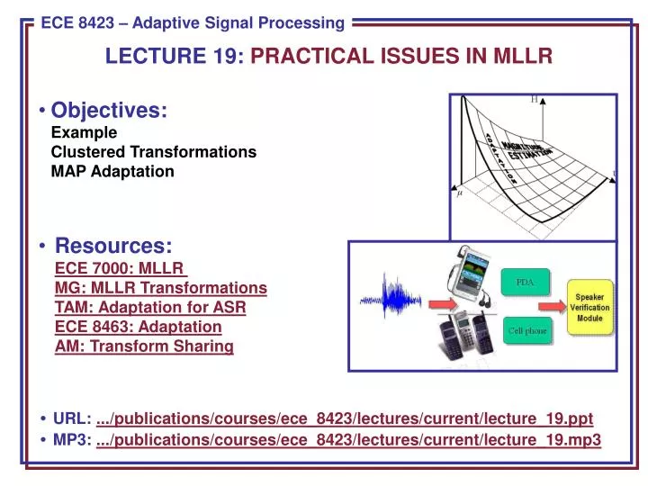
LECTURE 19: PRACTICAL ISSUES IN MLLR. Objectives: Example Clustered Transformations MAP Adaptation Resources: ECE 7000: MLLR MG: MLLR Transformations TAM: Adaptation for ASR ECE 8463: Adaptation AM: Transform Sharing.

E N D
LECTURE 19: PRACTICAL ISSUES IN MLLR • Objectives:ExampleClustered TransformationsMAP Adaptation • Resources:ECE 7000: MLLR MG: MLLR TransformationsTAM: Adaptation for ASRECE 8463: AdaptationAM: Transform Sharing • URL: .../publications/courses/ece_8423/lectures/current/lecture_19.ppt • MP3: .../publications/courses/ece_8423/lectures/current/lecture_19.mp3
MLLR Example • Let’s begin with a simple example involving a single state and a two-dimensional feature vector: • We observe two new data points: • We can estimate the new mean and covariance from these (noting that it is a noisy estimate because there are only two points): • Recall we assumed a diagonal covariance matrix, and derived an equation for the estimate of the elements of the transformation matrix: • Let’s assume the state occupancies are:These are arbitrary and would normally be accumulated during training of the model and represent the probability of being in state 1 at time t = 1 and 2.
MLLR Example (Cont.) • Then: • Recall our extended mean vector: • We can compute Z: • For a diagonal covariance, we defined G(i) as:
MLLR Example (Cont.) • Now we can solve for G(i)(there are i= 1, …,n of these, where n = 2):
MLLR Example (Cont.) • Next, we must solve for (G(i))-1. But there is a problem: The G(i) are singular (linearly dependent rows in this case). We typically use Singular Value Decomposition (from Numerical Recipes in C) to find a pseudo-inverse: • Now we can compute the components of W:
MLLR Example (Cont.) • We can finally compute the adapted means: • Recall that: • so MLLR has pushed the new mean very close to the observed data mean, but has done this using a transformation matrix.
Observations • The state occupancy probabilities determine the speed of adaptation, much like our adaptive filter. The more probable a state is, the more it will influence the overall calculation (another example of maximum likelihood). The larger the occupancy probabilities, the faster the adapted mean will move to the new mean. In general, the mean moves fairly quickly. • Question: If all we are doing is replacing the old mean with the new mean, why go through all this trouble? • The quality of the newmodel depends on theamount and richness of the new data. • Also, note that this isan unsupervised method,meaning the method doesnot need “truth-markings”of the adaptation data. • Many variants of the MLLRapproach exist today, includingsupervised versions.
Transform Sharing • Recall in our HMM, we had many states and manyGaussians per state. Transform sharing provides a means for dealing with small amounts of adaptation data under this scheme, even components that are not observed in the adaptation data can be adapted. • A common approach is the use of a binary regression class tree. • The leaves of the tree are termed as the "base regression classes“. • Each Gaussian mixture component of a model set belongs to a single base class. The tree has four base classes, C4, C5, C6, and C7. • During adaptation, occupation counts are accumulated for each of the base classes the dashed circles indicate clusters which have insufficient adaptation observations. • The details of this approach are beyond the scope of this course. However, the key point here is that the number of adaptation parameters can be controlled in a manner that is directly related to the overall likelihood.
Maximum A Posteriori (MAP) Adaptation • The MAP approach to adaptation attempts to maximize the posterior probability of the data given the model: • If we have no prior information, we can assume a uniform distribution for , and the MAP estimate is equivalent to the ML estimate. However, we can often estimate the prior from the training data. • The MAP estimate can be derived using a combination of the auxiliary function for the ML estimate and the prior: • If we assume the prior distribution of the parameters can be modeled as a multivariate Gaussian distribution, we can derive an expression for the MAP estimate of the new mean: • where is the number of observations in the adaptation data, is the existing mean estimated on the training data, is the ML estimate of the mean on the adaptation data, and is a balancing factor.
MLLR and MAP Comparison • We can gain some insight into these methods by examining their performance on a speech recognition task.
Summary • Demonstrated MLLR on a simple example. • Discussed some practical issues in its implementation. • Introduced MAP adaptation. • Compared the performance of the two on a speech recognition application. • Next: Take one more look at MLLR and MAP.