Flow Nets in River Channels: Understanding Aquifer Behavior

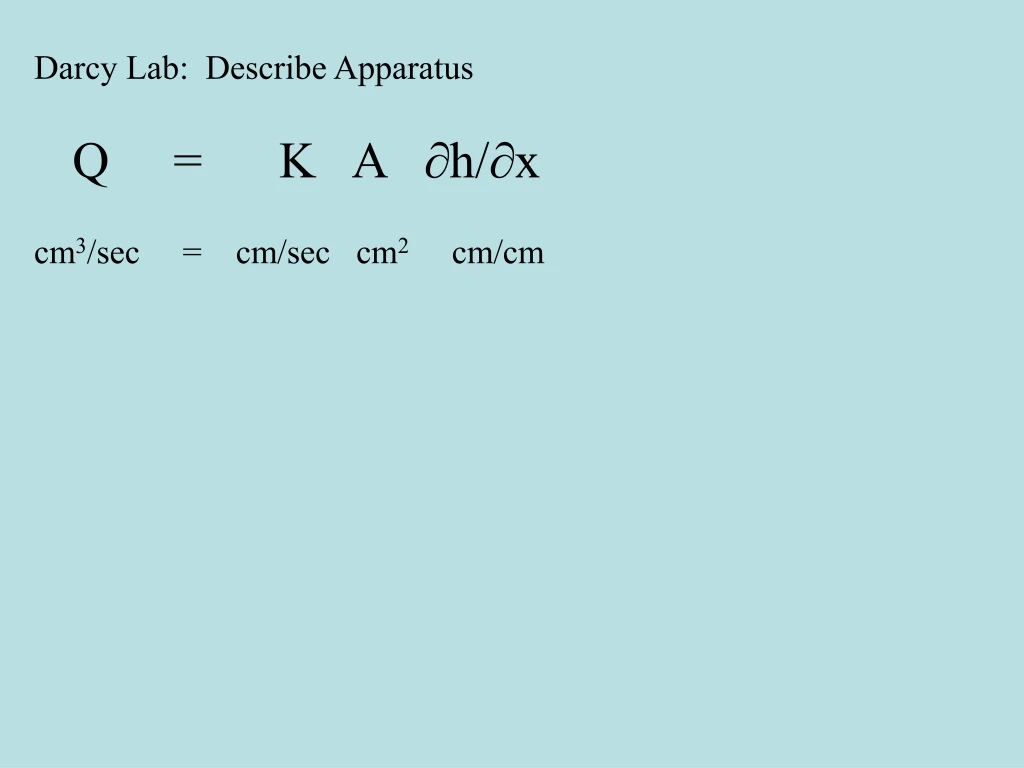
1. Darcy Lab: Describe Apparatus Q = K A ∂h/∂x cm3/sec = cm/sec cm2 cm/cm

2. River Channel Line Source Flow toward Pumping Well, next to river = line source = constant head boundary Plan view after Domenico & Schwartz (1990)

3. Flow Nets: Set of intersecting Equipotential lines and Flowlines Flowlines= Streamlines = Instantaneous flow directions Pathlines= Actual particle path Pathlines ≠ Flowlines for transient flow Flowlines | to Equipotential surface if K is isotropic Can be conceptualized in 3D

4. Flow Net Rules: Flowlines are perpendicular to equipotential lines (isotropic case) Spacing between equipotential lines L: If spacing between lines is constant, then K is constant In general K1 m1/L1 = K2 m2/L2where m = x-sect thickness of aquifer; L = distance between equipotential lines For layer of const thickness, K1/L1 ~ K2/L2 No Flow Boundaries Equipotential lines meet No Flow boundaries at right angles Flowlines are tangent to such boundaries (// flow) Constant Head Boundaries Equipotential lines are parallel to constant head boundaries Flow is perpendicular to constant head boundary

5. FLOW NETS Impermeble Boundary Constant Head Boundary Water Table Boundary after Freeze & Cherry

6. MK Hubbert 1903-1989 http://photos.aip.org/

7. MK Hubbert (1940) http://www.wda-consultants.com/java_frame.htm?page17

8. Consider piezometers emplaced near hilltop & near valley MK Hubbert (1940) http://www.wda-consultants.com/java_frame.htm?page17

9. Fetter, after Hubbert (1940)

10. Fetter, after Hubbert (1940)

11. Cedar Bog, OH

12. Piezometer Cedar Bog, Ohio

13. Topographic Highs tend to be Recharge Zones h decreases with depth Water tends to move downward => recharge zone Topographic Lows tend to be Discharge Zones h increases with depth Water will tend to move upward => discharge zone It is possible to have flowing well in such areas, if case the well to depth where h > h@ sfc. Hinge Line: Separates recharge (downward flow) & discharge areas (upward flow). Can separate zones of soil moisture deficiency & surplus (e.g., waterlogging). Topographic Divides constitute Drainage Basin Divides for Surface water e.g., continental divide Topographic Divides may or may not be GW Divides

14. Bluegrass Spring Criss

17. MK Hubbert (1940) http://www.wda-consultants.com/java_frame.htm?page17

18. Equipotential Lines Lines of constant head. Contours on potentiometric surface or on water tablemap => Equipotential Surface in 3D Potentiometric Surface: ("Piezometric sfc") Map of the hydraulic head; Contours are equipotential lines Imaginary surface representing the level to which water would rise in a nonpumping well cased to an aquifer, representing vertical projection of equipotential surface to land sfc. Vertical planes assumed; no vertical flow: 2D representation of a 3D phenomenon Concept rigorously valid only for horizontal flow w/i horizontal aquifer Measure w/ Piezometers= small dia non-pumping well with short screen- can measure hydraulic head at a point (Fetter, p. 134)

19. How do we know basic flownet picture is correct?

20. How do we know basic flownet picture is correct? Mathematical solutions (Toth, 1962, 1963) Numerical Simulations Data

21. Basin Geometry: Sinusoidal water table on a regional topo slope Toth (1962, 1963) h(x, z0) = z0 + Bx/L + b sin (2px/l) constant + regional slope + local relief B

22. Basin Geometry: Sinusoidal water table on a regional topo slope Toth (1962, 1963) h(x, z0) = z0 + Bx/L + b sin (2px/l) constant + regional slope + local relief Solve Laplace’s equation Simulate nested set of flow systems e.g., D&S How do we get q?

23. Discharge Recharge No Flow No Flow No Flow Regional flow pattern in an area of sloping topography and water table. Fetter, after Toth (1962) JGR67, 4375-87.

24. Systems Local Flow Intermediate Flow System Regional Flow System Australian Government after Toth 1963

25. Conclusions General slope causes regional GW flow system, If too small, get only local systems If the regional slope and relief are both significant, get regional, intermediate, and local GW flow systems. Local relief causes local systems. The greater the amplitude of the relief, the greater the proportion of the water in the local system If the regional slope and relief are both negligible, get flat water table often with waterlogged areas mostly discharged by ET For a given water table, the deeper the basin, the more important the regional flow High relief & deep basins promote deep circulation into hi T zones

26. End 24 Begin 25

27. FLOW NETS Flow Line Equipotential Line MK Hubbert 1903-1989 AIP Hubbert (1940) http://www.wda-consultants.com/java_frame.htm?page17

28. How do we know basic flownet picture is correct? Data Mathematical solutions (Toth, 1962, 1963) Numerical Simulations

29. Piezometer Cedar Bog, Ohio

30. Pierre Simon Laplace 1749-1827 Discharge Recharge No Flow No Flow No Flow Regional flow pattern in an area of sloping topography and water table. Fetter, after Toth (1962) JGR67, 4375-87.

31. Numerical Simulations Basically reproduce Toth’s patterns High K layers act as “pirating agents Refraction of flow lines tends to align flow parallel to hi K layer, and perpendicular to low K layers

32. Isotropic Systems Regular slope Sinusoidal slope Effect of Topography on Regional Groundwater Flow after Freeze and Witherspoon 1967 http://wlapwww.gov.bc.ca/wat/gws/gwbc/!!gwbc.html

33. Isotropic Aquifer Anisotropic Aquifer Kx: Kz = 10:1 after Freeze *& Witherspoon 1967

34. Layered Aquifers after Freeze *& Witherspoon 1967

35. Confined Aquifers Sloping Confining Layer Horizontal Confining Layer after Freeze *& Witherspoon 1967

36. Conclusions General slope causes regional GW flow system, If too small, get only local systems Local relief causes local systems. The greater the amplitude of the relief, the greater the proportion of the water in the local system If the regional slope and relief are both negligible, get flat water table often with waterlogged areas mostly discharged by ET If the regional slope and relief are both significant, get regional, intermediate, and local GW flow systems. For a given water table, the deeper the basin, the more important the regional flow High relief & deep basins promote deep circulation into hi T zones

37. Flow in a Horizontal Layers Case 1: Steady Flow in a Horizontal Confined Aquifer Darcy Velocity q: Flow/ unit width: Typically have equally-spaced equipotential lines

38. Case 2: Steady Flow in a Horizontal, Unconfined Aquifer Dupuit (1863) Assumptions: Grad h = slope of the water table Equipotential lines (planes) are vertical Streamlines are horizontal Flow/ unit width: m2/s Q’dx = -K h dh Dupuit Equation Fetter p. 164

39. h Impervious Base Steady flow No sources or sinks cf. Fetter p. 164

40. Better Approach Q’ = -K h dh/dx dQ’/dx = 0 continuity equation So: for one dimensional flow More generally, for an Unconfined Aquifer: Steady flow: No sources or sinks Laplace’s equation in h2 Steady flow with source term: Poisson Eq in h2 where w = recharge cm/sec cf. Fetter p. 167 F&C 189

41. Steady unconfined flow: with a source term Poisson Eq in h2 1-D Solution: Boundary conditions: @ x= 0 h= h1 ; @ x= L h= h2 cf. Fetter p. 167 F&C 189

42. w = 10-8 m/s K = 10-5 m/s @ x=0 h1 = 20m @ x=1000m h2 = 10m Unconfined flow with recharge w cf. Fetter p. 167 F&C 189

43. Finally, for unsteady unconfined flow: Boussinesq Eq. Sy is specific yield Fetter p. 150-1 For small drawdown compared to saturated thickness b: Linearized Boussinesq Eq. (Bear p. 408-9) Laplace’s Equation Steady flow Diffusion Equation Poisson’s Equation Steady Flow with Source or Sink

44. End Part II

47. Pierre Simon Laplace 1749-1827 Dibner Lib.

48. MK Hubbert 1903-1989 http://upload.wikimedia.org/wikipedia/en/f/f7/Hubbert.jpg

49. Leonhard Euler 1707 - 1783 wikimedia.org

50. Charles V. Theis 19-19 http://photos.aip.org/