Download
1 / 27
280 likes | 400 Views
Pixel Operations. 4c8 Dr. David Corrigan. Pixel Operations. This handout looks at the most basic type of image processing applications. These are simple point-wise operations of the form: I(h,k) is the input image g(h,k) if the output is some image processing function

E N D
Pixel Operations 4c8 Dr. David Corrigan
Pixel Operations • This handout looks at the most basic type of image processing applications. • These are simple point-wise operations of the form: • I(h,k) is the input image • g(h,k) if the output • is some image processing function • In a point-wise operation the output at (h,k) is dependent only on the value of the input (h,k) and not on the value of the input or output at any other location. • These types of operations are used mainly for image enhancement.
Matlab • Images are represented as a matrix • So G = 2.0 * I multiplies each pixel intensity by 2 and G = I + 10 increases the brightness by 2. • Point wise operations are fast and easy to implement in hardware.
Image Histograms • Records the number of pixels that have a particular intensity value • Typically displayed as a plot of frequency v intensity • Sometimes normalised so all the frequencies sum to 1 (ie. an approximation of the pdf of image intensities) • Colour images have 3D histograms but it is more common to use separate histograms for each colour channel. • Summarises where most of the pixels are so is useful for designing image enhancement operations • Matlab function hist() or imhist()
Image Histograms Y U V
Image Histograms It is also common to increase the bin width. Each frequency represents the number of pels in a particular range of intensities. Bin Width = 20 Bin Width = 1 Bin Width = 4
Contrast Enhancement & Clipping max intensity = 191 min intensity = 12 intensities fit full range
Contrast Enhancement & Clipping • used when you want to alter contrast or brightness of an image. • defines the alteration to the contrast. • c defines a global brightness change. • Clipping is necessary to ensure that all intensities in the output stay inside the valid range (ie. and ) but can also be used to eliminate contrast in very bright and dark regions. (ie. and )
Gamma Correction • Gamma Correction is a non-linear modification of image contrast. • If the contrast in the dark regions is increased and the contrast in the bright areas is increased • The opposite occurs if • Gamma Correction avoids the need for clipping so some contrast can be maintained in the dark/bright regions.
Histogram Equalisation • An automatic technique for image enhancement (no parameter choice required). • However, results are unpredictable and may look worse. • The idea is to alter the intensities so that the histogram is as flat as possible. • If the histogram contains a lot of pixels in a narrow range, it should be stretched out along the intensity range.
Histogram Equalisation i Levels H(i) Target H(i) m To have 16 pels at intensity 1, take all from I=1,2 and 8 from I = 3 and map onto intensity 1 because H(1) + H(2)+ 8 = 16 To have 16 pels at intensity 2 Take remainder (21-8)=13 at level 3, add to 3 from level 4 So intensity mapping is 1,2,3 -> 1; 3,4 ->2 etc etc
Histogram Equalisation Cumulative Histogram (scaled to fit axes) 1 0 Histogram
Histogram Equalisation • A problem arises because most bins will mapped onto more than one output bins. It is difficult to do this consistently. • Instead the cumulative histogram is used to design the mapping. Again the idea is to match the cumulative histogram to a target cumulative histogram. • The target cumulative histogram is a straight line, having a slope of 1/255, a max of 1 and a min of 0. This corresponds to a flat histogram. • Matlab function histeq()
Hist. Equalisation with CuF i Levels H(i) CuF(i) Target H(i) m Target CuF(i) m Match Bins of Cumulative Histogram to the closest bin in the target.
Hist. Equalisation with CuF i Levels H(i) CuF(i) Target H(i) m Target CuF(i) m Resulting transformation
Hist. Equalisation with CuF i Levels H(i) CuF(i) Target H(i) Target CuF(i) Output H(i) Output CuF(i)
Histogram Equalisation Matlab imadjdemo Try it
Histogram Equalisation Notice how the transformation between input and output relates to the cumulative histogram of the input.
Histogram Equalisation Histogram equalisation is more commonly applied to improve the contrast of medical images such as x-rays
Basic Segmentation (Thresholding) • Sometimes it is required to extract a part of an image which contains all the relevant in formation. If the information is contained in a limited band we can define a simple thresholding operation to segment the image in two. We choose and so that the part of the image he want fits inside this range. Eg. We might want to isolate the table to do some further analysis.
Intensity Based Segmentation Peak Corresponding to Table Histogram of Hue Segmented Table = 100, = 110 Extracted Table
Intensity Based Segmentation • The previous result can be improved by also incorporating a threshold on saturation • The condition for the table is now Histogram of Saturation Grayscale Representation of Saturation Segmented Table
Intensity Based Segmentation Segmentation with Hue alone Segmentation using Hue and Saturation
Matlab Implementation • Read the picture from file (eg. pic = imread(‘pool.jpg’);) • pic is a array storing the image in rgb format • pic(:,:,1) stores the red channel, pic(:,:,2) stores the green channel and pic(:,:,3) stores the blue channel. • Convert the image to the hsv and extract the hue and saturation channels colour space hsv = rgb2hsv(pic); hue = hsv(:,:,1); sat = hsv(:,:,2);
Matlab Implementation • Now we can define the segmentation operation mask = ((hue>100)&(hue<110)&(sat>128)); • To see the part of the image that has been segmented we create a new images as follows new_pic(:,:,1) = pic(:,:,1).*mask; new_pic(:,:,2) = pic(:,:,2).*mask; new_pic(:,:,3) = pic(:,:,3).*mask; • These lines create an image that is the same as the original image in the area of the table and is black in the background.
Matlab Implementation • People unfamiliar with Matlab get confused by the last part. In C++ it would be an if/else statement inside a for loop … for(int x = 0; x<width; x++){ for(int y = 0; y<height; y++){ for(int chan = 0; chan < 3; chan++){ if(mask[x][y]!=0) new_pic[x][y][chan]= pic[x][y][chan]; else new_pic[x][y][chan]= 0; } } }
Lab 1 • The first lab will get you to perform some of these pixel ops inside matlab. The segmentation code will help, however it is not complete! • In particular pay particular attention to the scaling of each colour channel • above we assumed that the hue channel was scaled between 0 and 360 and the saturation channel was scaled between 0 and 255. This will not be the case by default. • You will also have to learn what the best data type to use is int, float etc. You will also have to display your results as images and perhaps write them as files.