Download

1 / 104
1.07k likes | 1.09k Views
2. Foundations of FEM. 2.1 Direction stiffness method 2.2 Weighted residual method and Galerkin FEM 2.3 Rayleigh-Ritz method and Ritz FEM 2.4 Finite element method 2.5 Software for FEM 2.6 Examples. 2.1 Direction stiffness method. Spring system. Assume. Find nodal displacements.

E N D
2. Foundations of FEM 2.1 Direction stiffness method 2.2 Weighted residual method and Galerkin FEM 2.3Rayleigh-Ritz method and Ritz FEM 2.4 Finite element method 2.5 Software for FEM 2.6 Examples
2.1Direction stiffness method Spring system Assume Find nodal displacements Find reaction and spring forces.
Equilibrium equation Matrix form
Introduce displacement constraint Solve the equation, we obtain nodal displacements Reaction Spring forces
k1=500;k2=250;k3=2000;k4=1000; p=1000 K=[k1+k2 -k2 0; -k2 k2+k3+k4 -k4; 0 -k4 k4]; F=[0;0;p]; u=K\F u=[0;u] R=-k1*u(2)-k3*u(3) f1=k1*(u(2)-u(1)) f2=k2*(u(3)-u(2)) f3=k3*(u(3)-u(1)) f4=k4*(u(4)-u(3)) Tensile force
Direction stiffness method Element analysis Spring element Force equilibrium equation in X-axis for spring element
Apply pressure force on spring element From the relationship of force and displacement of spring, we have In matrix form,we have or Element stiffness matrix
Spring elements assemble into spring system Element 1 Element 2 Element 3 Element 4 assemble into spring system
By considering node equilibrium, we can simplify the right side
We obtain the same equilibrium equation as nodal equilibrium method Introduce displacement constraint and solve the equation, we can get the same answer.
ki=[500;250;2000;1000]; p=1000; eindex=[1 2;2 3;1 3; 3 4]; K=zeros(4,4); u=zeros(4,1); F=[0;0;0;p]; uid=[2 3 4]; for i=1:4 ke=ki(i)*[1 -1;-1 1]; K(eindex(i,:),eindex(i,:))=K(eindex(i,:),eindex(i,:))+ke; end KK=K(uid,uid); FF=F(uid); uu=KK\FF u(uid)=uu R=K(1,:)*u for i=1:4 ue=u(eindex(i,:)); fe=ki(i)*[-1 1]*ue end
Procedure for direction stiffness method • (1) Discrete • Element analysis to get element equilibrium equation. • Discrete and establish element assemble vectors. • (2) Assemble and solve • According to element assemble vectors, assemble element equations into system equation. • Apply forces and displacements constraints. • Solve equation to get unknown nodal displcements. • Compute reactions and element results.
Other representations for spring element Relationship of force and displcement Element equation Relationship of force and displcement Element equation
2.2 Weighted residual method and Galerkin FEM A straight bar loaded axial forces Linear distribution loadq=x. Concentrated force P=1. Elastic modulus E=1. cross-section area A=1. Length of bar L=1. Find the displacement of the right end of the bar.
Find analytic solution by material mechanics The relationship between force and deformation is Displacement generated by concentrated force P Displacement generated by linear distribution force q Total displacement at right end Substitute numeric value, we get the displacement at right end
Find analytic solution by elastic mechanics From infinitesimal equilibrium equation in X-axis, we have Infinitesimal force diagram The relationship of stress and strain The relationship of strain and displacement
From above formula, we obtain differential equation Displacement boundary Force boundary Solve the differential equation boundary value problem, we obtain the solution as The displacement at right end is
Integral statements equivalent to the differential equations D.E. Differential equation boundary value problem D.B.C. F.B.C. Equivalent integral statements D.B.C. F.B.C.
Weighted residual method 1. Point Collocation Method 2. Least Squares Method 3. Galerkin’s Method
One term in the trial function Assume displacement function as Satisfy D.B.C, we have Satisfy F.B.C, we have Therefore, the assumed displacement function written as The residual is The integration of the weighted residual is
1. Point Collocation Method The weighted function syms a x real; u=(1-2*a)*x+a*x^2; R=diff(u,x,2)+x; I=subs(R,x,0.5); a=solve(I); numeric(a)
2. Least Squares Method syms a x real; u=(1-2*a)*x+a*x^2; R=diff(u,x,2)+x; w=diff(R,a); I=int(w*R,0,1); a=solve(I); numeric(a)
3. Galerkin’s Method syms a x real; u=(1-2*a)*x+a*x^2; R=diff(u,x,2)+x; w=diff(u,a); I=int(w*R,0,1); a=solve(I); numeric(a)
x=0:0.1:1; u0=1.5*x-x.^3/6; a=-0.25;ucm=(1-2*a)*x+a*x.^2; a=-0.25;ulsm=(1-2*a)*x+a*x.^2; a=-5/16;ugm=(1-2*a)*x+a*x.^2; plot(x,u0,x,ucm,x,ulsm,x,ugm) legend('准确解','配点法','最小二乘法','Galerkin法') xlabel('x') ylabel('u') title('近似函数待定参数取1项')
Two terms in the trial function Assume displacement function as Satisfy D.B.C, we have Satisfy F.B.C, we have Therefore, the assumed displacement function written as The residual is The integration of the weighted residual is
1. Point Collocation Method The weighted function Take
syms a1 a2 x real; u=(1-2*a1-3*a2)*x+a1*x^2+a2*x^3; R=diff(u,x,2)+x; I1=subs(R,x,1/3); I2=subs(R,x,2/3); [a1,a2]=solve(I1,I2); numeric(a1), numeric(a2)
, syms a1 a2 x real; u=(1-2*a1-3*a2)*x+a1*x^2+a2*x^3 R=diff(u,x,2)+x; w1=diff(R,a1); w2=diff(R,a2); I1=int(w1*R,0,1); I2=int(w2*R,0,1); [a1,a2]=solve(I1,I2); numeric(a1), numeric(a2 2. Least Squares Method ,
3. Galerkin’s Method , syms a1 a2 x real; u=(1-2*a1-3*a2)*x+a1*x^2+a2*x^3; R=diff(u,x,2)+x; w1=diff(u,a1); w2=diff(u,a2); I1=int(w1*R,0,1); I2=int(w2*R,0,1); [a1,a2]=solve(I1,I2); numeric(a1), numeric(a2) , 。
Galerkin’s method applies to weak form By using integration by parts, we have Substitute into the equivalent integral statements, we have Substitute F.B.C, we have Natural boundary conditions
If we select weighted function that satisfies We obtain the equivalent weak form of differential equation D.B.C Weighted function must satisfies Essential boundary conditions
Assume weighted function w as virtual displacement From the relationship of stain and displacement, we can take as virtual strain For the problem, it has Therefore, the equivalent weak form can written as Virtual displacement principle Internal virtual work External virtual work by concentrated force External virtual work by linear distribution force
One term in the trial function Assume displacement function as Satisfies D.B.C, we have Therefore, the assume displacement function is written as For Galerkin’s method, weighted function is taken as It satisfies
syms a x real; %定义实数型符号变量a,x u=a*x; %定义u的近似函数 w=diff(u,a); %计算权函数 du=diff(u,x); %u对x的导数 dw=diff(w,x); %w对x的导数 I=int(-dw*du+w*x,0,1)+subs(w,x,1)*1; %计算残值的加权积分 a=solve(I); %求解确定参数 numeric(a) %得到数值形式解
Two terms in the trial function , Assume displacement function as , Satisfies D.B.C, we have Therefore, the assume displacement function is written as For Galerkin’s method, weighted function is taken as It satisfies
syms a1 a2 x real; %定义实数型符号变量a,x u=a1*x+a2*x^2; %定义u的近似函数 w1=diff(u,a1); %计算权函数 w2=diff(u,a2); %计算权函数 du=diff(u,x); %u对x的导数 dw1=diff(w1,x); %w1对x的导数 dw2=diff(w2,x); %w2对x的导数 I1=int(-dw1*du+w1*x,0,1)+subs(w1,x,1)*1; %计算残值的加权积分 I2=int(-dw2*du+w2*x,0,1)+subs(w2,x,1)*1; %计算残值的加权积分 [a1,a2]=solve(I1,I2); %求解确定参数 a1= numeric(a1),a2= numeric(a2) %得到数值形式解
Three terms in the trial function , , , Assume displacement function as , , , Satisfies D.B.C, we have Therefore, the assume displacement function is written as For Galerkin’s method, weighted function is taken as
syms a1 a2 a3 x real; %定义实数型符号变量a,x u=a1*x+a2*x^2+a3*x^3; %定义u的近似函数 w1=diff(u,a1); %计算权函数 w2=diff(u,a2); %计算权函数 w3=diff(u,a3); %计算权函数 du=diff(u,x); %u对x的导数 dw1=diff(w1,x); %w1对x的导数 dw2=diff(w2,x); %w2对x的导数 dw3=diff(w3,x); %w3对x的导数 I1=int(-dw1*du+w1*x,0,1)+subs(w1,x,1)*1; %计算残值的加权积分 I2=int(-dw2*du+w2*x,0,1)+subs(w2,x,1)*1; %计算残值的加权积分 I3=int(-dw3*du+w3*x,0,1)+subs(w3,x,1)*1; %计算残值的加权积分 [a1,a2,a3]=solve(I1,I2,I3); %求解确定参数 a1= numeric(a1),a2= numeric(a2),a3= numeric(a3) %得到数值形式解
x=0:0.1:1; u0=1.5*x-x.^3/6; u1=4/3*x; u2=19/12*x-0.25*x.^2; u3=1.5*x-x.^3/6; plot(x,u0,x,u1,x,u2,x,u3) legend('精确解','近似解参数1个','近似解参数2个','近似解参数3个') xlabel('x') ylabel('u') title('Galerkin法-弱形式')
Assume displacement function as Satisfies D.B.C, we have Therefore, the assumed displacement function is where
Apply Galerkin method, weighted function and its derivatives are
The derivative of assumed displacement function The weighted residual equations
In matrix form , Computation of matrix and vectors
Finally, obtain the equation as Solve the equation obtain the results as
syms a1 a2 a3 a4 x real; %定义实数型符号变量a1,a2,x h1=[4*x;2-4*x;0;0]; %将三分段函数用列向量形式表示 h2=[0;4*x-1;3-4*x;0]; %将三分段函数用列向量形式表示 h3=[0;0;4*x-2;4-4*x]; %将三分段函数用列向量形式表示 h4=[0;0;0;4*x-3]; %将三分段函数用列向量形式表示 u=a1*h1+a2*h2+a3*h3+a4*h4; %定义u的近似函数 w1=diff(u,a1); %计算权函数 w2=diff(u,a2); %计算权函数 w3=diff(u,a3); %计算权函数 w4=diff(u,a4); %计算权函数 du=diff(u,x); %u对x的导数 dw1=diff(w1,x); %w1对x的导数 dw2=diff(w2,x); %w2对x的导数 dw3=diff(w3,x); %w3对x的导数 dw4=diff(w4,x); %w4对x的导数
I1=int(-dw1(1)*du(1)+w1(1)*x,0,1/4)... +int(-dw1(2)*du(2)+w1(2)*x,1/4,2/4)... +int(-dw1(3)*du(3)+w1(3)*x,2/4,3/4)... +int(-dw1(4)*du(4)+w1(4)*x,3/4,1); %计算残值的加权积分 I2=int(-dw2(1)*du(1)+w2(1)*x,0,1/4)... +int(-dw2(2)*du(2)+w2(2)*x,1/4,2/4)... +int(-dw2(3)*du(3)+w2(3)*x,2/4,3/4)... +int(-dw2(4)*du(4)+w2(4)*x,3/4,1); %计算残值的加权积分 I3=int(-dw3(1)*du(1)+w3(1)*x,0,1/4)... +int(-dw3(2)*du(2)+w3(2)*x,1/4,2/4)... +int(-dw3(3)*du(3)+w3(3)*x,2/4,3/4)... +int(-dw3(4)*du(4)+w3(4)*x,3/4,1); %计算残值的加权积分 I4=int(-dw4(1)*du(1)+w4(1)*x,0,1/4)... +int(-dw4(2)*du(2)+w4(2)*x,1/4,2/4)... +int(-dw4(3)*du(3)+w4(3)*x,2/4,3/4)... +int(-dw4(4)*du(4)+w4(4)*x,3/4,1)+1; %计算残值的加权积分 [a1,a2,a3,a4]=solve(I1,I2,I3,I4); %求解确定参数 numeric(a1), numeric(a2), numeric(a3), numeric(a4)