Download
1 / 19
190 likes | 285 Views
Off-axis Simulations. Peter Litchfield, Minnesota. What has been simulated? Will the experiment work? Can we choose a technology based on simulations? Still very much work to be done, it is only early days yet. What has been simulated?. A somewhat idealized RPC detector

E N D
Off-axis Simulations Peter Litchfield, Minnesota • What has been simulated? • Will the experiment work? • Can we choose a technology based on simulations? • Still very much work to be done, it is only early days yet.
What has been simulated? • A somewhat idealized RPC detector • A more realistic scintillator detector • Liquid • Solid • Three analyses have been written up and are available as off-axis notes • Fermilab (RPCs) • SLAC (RPCs) • Minnesota (Scintillator) • I am most familiar with the scintillator analysis and I will describe this in more detail. The RPC analyses are similar in principle and obtain broadly similar results.
Liquid Scintillator Detector Simulation • Used the MINOS simulation framework. • Used NEUGEN3 for the event generation. • Simulated a detector ~ 30m x 15m x190m, absorber density = 0.7 g/cc, readout planes separated by 0.33 of a radiation length, 50ktons total weight. • Liquid scintillator strips were 4cm wide x 2.9cm thick x 15m long, read out by a looped fiber to an APD pixel. • Light collection and attenuation simulated according to measurements of prototype 15m fibers and the experience of MINOS. • Light level set to average 35 photo-electrons read out from a normal minimum ionizing particle at the far end of a strip. • APD readout, including noise, simulated according to the experience of CMS.
Event Samples • A detector at the proposed site, 820km from Fermilab and 12km off-axis was simulated • Neutrino events were generated with a flat event distribution from 100 MeV to 20 GeV and uniformly throughout the detector. Equal numbers of events were generated between 100 MeV and 3 Gev and 3 GeV and 20 GeV. • Charged current , charged current e and neutral current events were generated separately • Beam spectra for the site were imposed by weighting the events • A 50kton detector, run for 5 years with 41020 pot/year • Oscillations with m2=0.0025, sin2223=1 and sin2213=0.1 were assumed. • Samples of ~0.5M events in each category were used to define the analysis procedure and cuts and a similar, separate, sample to calculate the event selection efficiencies.
Event Reconstruction • Firstly a clustering algorithm was applied which collected all hits which were within 2m of their nearest neighbour. • Three hits were required to establish a cluster. • The clusters in the two views were matched and the largest matched clusters in the two views taken as the event. Usually there was only one cluster in each view. • Using the reconstructed position of the event in space the hit pulse heights were corrected for attenuation • A straight line was fitted to the event hits in the two views and the residuals, unweighted and weighted by the pulse height were calculated • Secondly the dominant track in the event was found using a Hough Transform method. • A straight line was then fitted to the hits assigned to this track and the pulse height weighted and unweighted residuals calculated
Event selection A series of cuts were made on distributions where the background events can be separated reasonably cleanly from the electron events. Pdfs for the different event classes were calculated from distributions where the events had substantial overlaps. A likelihood ratio was calculated for the oscillated electron events versus the muon CC, neutral current and electron beam events. Cuts were applied to these distributions to produce an electron CC event sample and the amount of background from the other categories calculated. The scintillator and RPC analyses are similar in principle but different cut and pdf variables were used.
Events Truth neutrino energy after oscillations Unoscillated beam events as a function of truth neutrino energy Number of hits outside fiducial volume (50cm lateral, 200cm longitudinal). Events with more than 2 hits outside are rejected. 84% efficiency Truth neutrino energy distribution after reconstruction
Cuts Total pulse height Rejects high energy e CC events and low visible energy events Event length Rejects CC events Fraction of hits in the Hough track Selects low-y or quasi-elastic events Number of planes in the Hough track. Requires a good track
Cuts Hits/plane on the Hough track Selects “fuzzy” electron tracks Angle of Hough track to beam Rejects a few mis-reconstructed events
Likelihood pdfs (sample) Angle of Hough track to beam versus total pulse height Total pulse height v pulse height weighted residual to fitted line
Likelihood Ratios e oscillated versus CC e oscillated versus NC e oscillated versus e beam Select as e events those to the right of the cut line in all three plots
Cut signal CC NC beam e generated events 474517 461891 488439 beam weighted 18606 5692 394 beam weighted +osc 6434 5692 394 603 events with good clusters 6105 3530 344 538 fiducial volume 3937 3216 288 486 event length 776 2155 121 417 total ph 364 549 46.0 334 planes in Hough track 330 425 42.2 312 Hough fraction 31.6 20.0 16.0 141 Hough hits/plane 5.2 15.6 15.6 136 Beam angle 2.6 14.2 15.2 132 Numbers Figure of Merit = Signal/Background = 25.30.4
RPC or Scintillator? • Simulations in principle can help in the choice of technology • BUT the simulations need to be comparable in everything but the technology choice. • Not the case at present, the RPC simulation is less complete than the scintillator, we are working towards a true comparison for the proposal. • An RPC with one dimensional readout is in principle very similar to a scintillator strip with no pulse height measurement, the differences are in the details of the readout. • RPCs can have two dimensional readout of a single active plane which can help in the pattern recognition and particle counting • Scintillator strips can measure pulse height which counts minimum ionizing particle equivalents • Which gives most gain is a detailed problem to which we do not yet have an answer.
Conclusions • Simulations show that 50kton detector constructed either with RPC or scintillator at this site and with this beam flux will give a very strong signal for sin2213=0.1 and m2=0.0025 eV2. • The current simulations would give a 90% confidence limit just based on statistics of ~1/10th of this value with this detector and beam flux. • The simulations are far from final, better algorithms may be developed. • Currently the simulations cannot differentiate between the technologies, more complete and comparable simulations are needed which are being worked on.