Download
1 / 11
110 likes | 276 Views
Pest Management Modeling. PESTS. CAUSE DAMAGE TO CROPS ONE-THIRD OF EVERYTHING GROWN 4 BILLION DOLLARS. CURRENT CONTROL METHODS. MAINLY CHEMICAL INSECTICIDES DISADVANTAGES PEST RESISTANCE NON-SELECTIVE PEST SURGES ENVIRONMENTAL DAMAGE. INTEGRATED PEST MANAGEMENT (IPM).

E N D
PESTS • CAUSE DAMAGE TO CROPS • ONE-THIRD OF EVERYTHING GROWN • 4 BILLION DOLLARS
CURRENT CONTROL METHODS • MAINLY CHEMICAL INSECTICIDES • DISADVANTAGES • PEST RESISTANCE • NON-SELECTIVE • PEST SURGES • ENVIRONMENTAL DAMAGE
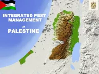
INTEGRATED PEST MANAGEMENT (IPM) “THE GOAL OF IPM RESEARCH IS TO DESIGN SYSTEMS FOR CONTROLLING PEST DAMAGE THAT ARE APPROPRIATE FOR THE SITE WHILE REDUCING RELIANCE ON CHEMICAL PESTICIDES” -USDA
GROWER CROP PEST NATURAL CONTROL ENVIRONMENT
MATHEMATICAL MODELING • OPTIMIZE CHEMICAL CONTROL • SCHEDULE PEST APPLICATION • REALEASE STERILE MALES • PREDICT PEST POPULATION • CROP SYSTEMS DESIGNS
Crop System Design H=number of prey P=predator population a=prey’s birth rate b=predator’s attack rate c=predator’s death rate d=efficiency which prey are converted to predators t=length of time lag Lotka-Volterra • Subscripts refer to the 2 systems • Patchiness would not increase stability
Crop System Design Cont. Functional Response b=time predator takes to handle prey G(h)=average number of prey eaten in a random patch S(h)=average amount of time spent search in a random patch f(h)/h=risk each prey has of being eaten Stable for Holling’s Type III
Crop System Design Cont. 2 Species of Pests: Assume is the time spent searching in area 1: Predator switches back and forth between the two prey species. Ni=prey species ai=rate predator searches for prey i bi=handling time H=number of prey i
CONCLUSIONS • MATH OFFERS A WIDE VARIETY OF TOOLS • MOSTLY THEORETICAL • UNLIKELY GENERAL THEORY CREATED • EACH PROBLEM REQUIRES IN-DEPTH STUDY • USED INCREASINGLY IN THE FUTURE AS PESTICIDE USE BECOMES LIMITED
References Chatterjee, Samprit. A Mathematical Model for Pest Control. Biometrics 1973, 29, 727-734. Murdoch, William W.; Briggs, Cheryl J.; Theory for Biological Control: Recent Developments. Ecology 1996, 77, 2001-2013. Murdoch, William; Diversity, Complexity, Stability and Pest Control. The Journal of Applied Ecology 1975, 12, 795-807. Plant, Richard; Mangel, Mark. Modeling and Simulation in Agricultural Pest Management. SIAM Review1987, 29, 235-261. Rafikov; Balthazar, Jose Manoel; Optimal Pest Control Problem in Population Dynamics. Computational and Applied Mathematics 2005, 24. U.S. Department of Agriculture Home Page. http://www.usda.gov (accessed Dec 2006).