Download
1 / 97
970 likes | 993 Views
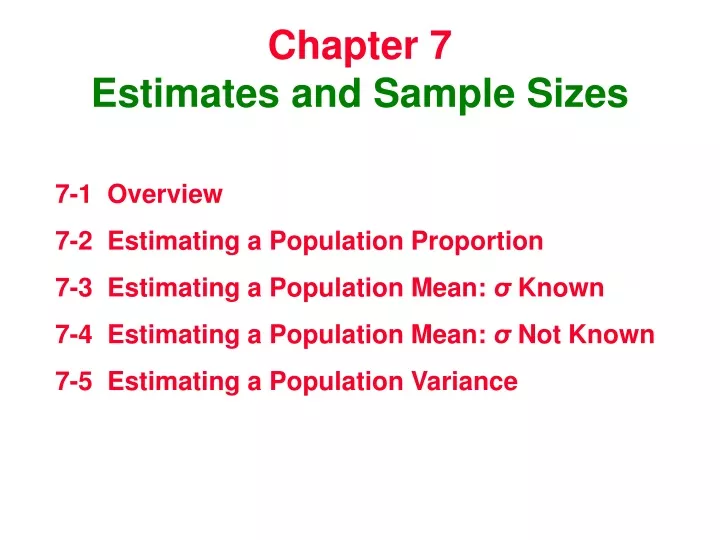
Chapter 7 Estimates and Sample Sizes. 7-1 Overview 7-2 Estimating a Population Proportion 7-3 Estimating a Population Mean: σ Known 7-4 Estimating a Population Mean: σ Not Known 7-5 Estimating a Population Variance. Section 7-1 Overview. Created by Erin Hodgess, Houston, Texas

E N D
Chapter 7Estimates and Sample Sizes 7-1 Overview 7-2 Estimating a Population Proportion 7-3 Estimating a Population Mean: σ Known 7-4 Estimating a Population Mean: σ Not Known 7-5 Estimating a Population Variance
Section 7-1 Overview Created by Erin Hodgess, Houston, Texas Revised to accompany 10th Edition, Tom Wegleitner, Centreville, VA
Overview This chapter presents the beginning of inferential statistics. • The two major applications of inferential statistics involve the use of sample data to (1) estimate the value of a population parameter, and (2) test some claim (or hypothesis) about a population. • We introduce methods for estimating values of these important population parameters: proportions, means, and variances. • We also present methods for determining sample sizes necessary to estimate those parameters.
Section 7-2 Estimating a Population Proportion Created by Erin Hodgess, Houston, Texas Revised to accompany 10th Edition, Tom Wegleitner, Centreville, VA
Key Concept In this section we present important methods for using a sample proportion to estimate the value of a population proportion with a confidence interval. We also present methods for finding the size of the sample needed to estimate a population proportion.
Requirements for Estimating a Population Proportion • 1. The sample is a simple random sample. • 2. The conditions for the binomial distribution are satisfied. (See Section 5-3.) • 3. There are at least 5 successes and 5 failures.
p= population proportion Notation for Proportions ˆ p= x n sample proportion of xsuccesses in a sample of size n (pronounced ‘p-hat’) ˆ ˆ q = 1 - p=sampleproportion of failures in a sample size of n
Definition A point estimate is a single value (or point) used to approximate a population parameter.
Definition The sample proportion p is the best point estimate of the population proportion p. ˆ
Example: 829 adult Minnesotans were surveyed, and 51% of them are opposed to the use of the photo-cop for issuing traffic tickets. Using these survey results, find the best point estimate of the proportion of all adult Minnesotans opposed to photo-cop use. Because the sample proportion is the best point estimate of the population proportion, we conclude that the best point estimate of p is 0.51. When using the survey results to estimate the percentage of all adult Minnesotans that are opposed to photo-cop use, our best estimate is 51%.
Definition A confidence interval (or interval estimate) is a range (or an interval) of values used to estimate the true value of a population parameter. A confidence interval is sometimes abbreviated as CI.
Definition A confidence level is the probability 1- (often expressed as the equivalent percentage value) that is the proportion of times that the confidence interval actually does contain the population parameter, assuming that the estimation process is repeated a large number of times. (The confidence level is also called degree of confidence, or the confidence coefficient.) Most common choices are 90%, 95%, or 99%. ( = 10%), ( = 5%), ( = 1%)
Example: 829 adult Minnesotans were surveyed, and 51% of them are opposed to the use of the photo-cop for issuing traffic tickets. Using these survey results, find the 95% confidence interval of the proportion of all adult Minnesotans opposed to photo-cop use. “We are 95% confident that the interval from 0.476 to 0.544 does contain the true value of p.” This means if we were to select many different samples of size 829 and construct the corresponding confidence intervals, 95% of them would actually contain the value of the population proportion p.
Using Confidence Intervals for Comparisons Do not use the overlapping of confidence intervals as the basis for making formal and final conclusions about the equality of proportions.
Critical Values 1. We know from Section 6-6 that under certain conditions, the sampling distribution of sample proportions can be approximated by a normal distribution, as in Figure 7-2, following. 2. Sample proportions have a relatively small chance (with probability denoted by ) of falling in one of the red tails of Figure 7-2, following. 3. Denoting the area of each shaded tail by /2, we see that there is a total probability of that a sample proportion will fall in either of the two red tails.
Critical Values 4. By the rule of complements (from Chapter 4), there is a probability of 1- that a sample proportion will fall within the inner region of Figure 7-2, following. 5. The z score separating the right-tail is commonly denoted by z /2 and is referred to as a critical value because it is on the borderline separating sample proportions that are likely to occur from those that are unlikely to occur.
z2 The Critical Value Figure 7-2
Notation for Critical Value The critical valuez/2is the positivezvalue that is atthe vertical boundary separating an area of/2in the right tail of the standard normal distribution.(The value of –z/2is at the vertical boundary for thearea of/2in the left tail.) The subscript/2issimply a reminder that thezscore separates an areaof /2in the right tail of the standard normal distribution.
Definition A critical value is the number on the borderline separating sample statistics that are likely to occur from those that are unlikely to occur. The number z/2 is a critical value that is a z score with the property that it separates an area of /2in the right tail of the standard normal distribution. (See Figure 7-2).
z2 -z2 Critical Values Finding z2 for a 95% Confidence Level = 5% 2 = 2.5% = .025
z2 = 1.96 Finding z2 for a 95% Confidence Level - cont = 0.05 Use Table A-2 to find a z score of 1.96
Definition When data from a simple random sample are used to estimate a population proportion p, the margin of error, denoted by E, is the maximum likely (with probability 1 – ) difference between the observed proportion p and the true value of the population proportion p. The margin of error E is also called the maximum error of the estimate and can be found by multiplying the critical value and the standard deviation of the sample proportions, as shown in Formula 7-1, following. ˆ
ˆ ˆ z pq E= a / 2 n Margin of Error of the Estimate of p Formula 7-1
ˆ p ˆ p p – E < < + E E= ˆ ˆ z pq a / 2 n Confidence Interval for Population Proportion where
ˆ p ˆ p p – E < < + E p + E (p – E, p + E) ˆ ˆ Confidence Interval for Population Proportion - cont ˆ
Round-Off Rule for Confidence Interval Estimates of p • Round the confidence interval limits for p to three significant digits.
pq n ˆ ˆ Procedure for Constructing a Confidence Interval for p • Verify that the required assumptions are satisfied. (The sample is a simple random sample, the conditions for the binomial distribution are satisfied, and the normal distribution can be used to approximate the distribution of sample proportions because np 5, and nq 5 are both satisfied.) 2. Refer to Table A-2 and find the critical value z/2 that corresponds to the desired confidence level. 3. Evaluate the margin of error E =
Procedure for Constructing a Confidence Interval for p - cont 4. Using the value of the calculated margin of error, E and the value of the sample proportion, p, find the values of p – Eand p + E. Substitute those values in the general format for the confidence interval: ˆ ˆ ˆ ˆ ˆ p – E < p < p + E 5. Round the resulting confidence interval limits to three significant digits.
Example: 829 adult Minnesotans were surveyed, and 51% of them are opposed to the use of the photo-cop for issuing traffic tickets. Use these survey results. a)Find the margin of errorE that corresponds to a 95% confidence level. b) Find the 95% confidence interval estimate of the population proportion p. c) Based on the results, can we safely conclude that the majority of adult Minnesotans oppose use the the photo-cop?
Example: 829 adult Minnesotans were surveyed, and 51% of them are opposed to the use of the photo-cop for issuing traffic tickets. Use these survey results. a)Find the margin of errorE that corresponds to a 95% confidence level. ˆ ˆ First, we check for assumptions. We note that np = 422.79 5, and nq = 406.21 5. ˆ ˆ Next, we calculate the margin of error. We have found thatp=0.51, q= 1 – 0.51 = 0.49, z2= 1.96, and n = 829. E = 1.96 (0.51)(0.49) 829 E=0.03403
Example: 829 adult Minnesotans were surveyed, and 51% of them are opposed to the use of the photo-cop for issuing traffic tickets. Use these survey results. b)Find the 95% confidence interval for the population proportion p. We substitute our values from Part a to obtain: 0.51 – 0.03403 < p < 0.51 + 0.03403, 0.476 < p < 0.544
Example: 829 adult Minnesotans were surveyed, and 51% of them are opposed to the use of the photo-cop for issuing traffic tickets. Use these survey results. c)Based on the results, can we safely conclude that the majority of adult Minnesotans oppose use of the photo-cop? Based on the survey results, we are 95% confident that the limits of 47.6% and 54.4% contain the true percentage of adult Minnesotans opposed to the photo-cop. The percentage of opposed adult Minnesotans is likely to be any value between 47.6% and 54.4%. However, a majority requires a percentage greater than 50%, so we cannot safely conclude that the majority is opposed (because the entire confidence interval is not greater than 50%).
Sample Size Suppose we want to collect sample data with the objective of estimating some population. The question is how many sample items must be obtained?
ˆ ˆ p q z E= a / 2 n (solve for n by algebra) ˆ ˆ Z ()2 a / 2 p q n = E 2 Determining Sample Size
ˆ When an estimate of p is known: ˆ z ˆ ()2 p q a / 2 n = Formula 7-2 E 2 ˆ When no estimate of p is known: z ()2 a / 2 Formula 7-3 0.25 n = E 2 Sample Size for Estimating Proportion p
Example: Suppose a sociologist wants to determine the current percentage of U.S. households using e-mail. How many households must be surveyed in order to be 95% confident that the sample percentage is in error by no more than four percentage points? a) Use this result from an earlier study: In 1997, 16.9% of U.S. households used e-mail (based on data from The World Almanacand Book of Facts). b) Assume that we have no prior information suggesting a possible value of p. ˆ
ˆ ˆ n = [za/2 ]2p q E2 To be 95% confident that our sample percentage is within four percentage points of the true percentage for all households, we should randomly select and survey 338 households. = [1.96]2(0.169)(0.831) 0.042 = 337.194 = 338 households Example: Suppose a sociologist wants to determine the current percentage of U.S. households using e-mail. How many households must be surveyed in order to be 95% confident that the sample percentage is in error by no more than four percentage points? a) Use this result from an earlier study: In 1997, 16.9% of U.S. households used e-mail (based on data from The World Almanacand Book of Facts).
n = [za/2 ]2• 0.25 E2 Example: Suppose a sociologist wants to determine the current percentage of U.S. households using e-mail. How many households must be surveyed in order to be 95% confident that the sample percentage is in error by no more than four percentage points? b) Assume that we have no prior information suggesting a possible value of p. ˆ With no prior information, we need a larger sample to achieve the same results with 95% confidence and an error of no more than 4%. = (1.96)2 (0.25) 0.042 = 600.25 = 601 households
Finding the Point Estimate and E from a Confidence Interval Point estimate of p: p=(upper confidence limit) + (lower confidence limit) 2 ˆ ˆ Margin of Error: E = (upper confidence limit) — (lower confidence limit) 2
Recap In this section we have discussed: • Point estimates. • Confidence intervals. • Confidence levels. • Critical values. • Margin of error. • Determining sample sizes.
Section 7-3 Estimating a Population Mean: Known Created by Erin Hodgess, Houston, Texas Revised to accompany 10th Edition, Tom Wegleitner, Centreville, VA
Key Concept This section presents methods for using sample data to find a point estimate and confidence interval estimate of a population mean. A key requirement in this section is that we know the standard deviation of the population.
Requirements 1. The sample is a simple random sample. (All samples of the same size have an equal chance of being selected.) 2. The value of the population standard deviation is known. 3. Either or both of these conditions is satisfied: The population is normally distributed or n > 30.
The sample mean xis the best point estimate of the population mean µ. Point Estimate of the Population Mean
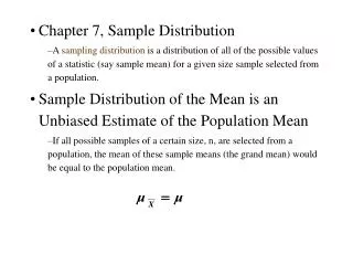
Sample Mean • For all populations, the sample mean x is an unbiased estimator of the population mean , meaning that the distribution of sample means tends to center about the value of the population mean . 2. For many populations, the distribution of samplemeansxtends to be more consistent (with less variation) than the distributions of other sample statistics.
Example: A study found the body temperatures of 106 healthy adults. The sample mean was 98.2 degrees and the sample standard deviation was 0.62 degrees. Find the point estimate of the population mean of all body temperatures. Because the sample mean x is the best point estimate of the population mean , we conclude that the best point estimate of the population mean of all body temperatures is 98.20o F.
Definition The margin of error is the maximum likely difference observed between sample mean x and population mean µ, and is denoted by E.
E = z/2 •Formula 7-4 n Formula Margin of Error Margin of error for mean (based on known σ)
x – E < µ < x+ E x+ E (x –E, x + E) Confidence Interval estimate of the Population Mean µ (with Known) or or
Definition The two values x – E and x + E are called confidence interval limits.