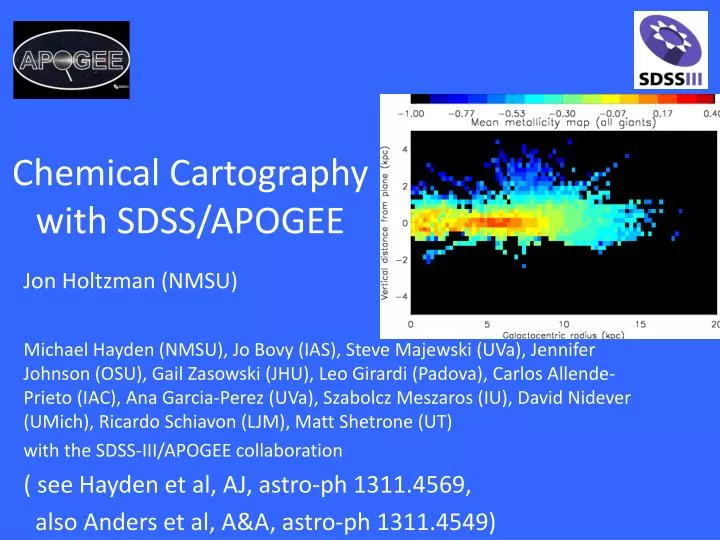
Chemical Cartography with SDSS/APOGEE

1. Chemical Cartography with SDSS/APOGEE Jon Holtzman (NMSU) Michael Hayden (NMSU), Jo Bovy (IAS), Steve Majewski (UVa), Jennifer Johnson (OSU), Gail Zasowski (JHU), Leo Girardi (Padova), Carlos Allende-Prieto (IAC), Ana Garcia-Perez (UVa), SzabolczMeszaros (IU), David Nidever (UMich), Ricardo Schiavon (LJM), Matt Shetrone (UT) with the SDSS-III/APOGEE collaboration ( see Hayden et al, AJ, astro-ph 1311.4569, also Anders et al, A&A, astro-ph 1311.4549)

2. APOGEE at a Glance • SDSS-III -- One of four experiments (BOSS/APOGEE until 2014) • Bright time 2011.Q2 - 2014.Q2 • 300 fiber, R ≥ 22,500, cryogenic spectrograph, 7 deg2 FOV • H-band: 1.51-1.69m AH /AV ~ 1/6 • S/N ≥ 100/pixel @ H=12.2 for 3-hr total integration • RV uncertainty spec. < 0.5 km/s, 3-hr; actual<~100 m/s, 1-hr • 0.1 dex precision abundances for ~15 chemical elements(including Fe, C, N, O, -elements, odd-Z elements, iron peak elements, possibly even neutron capture) • 105 2MASS-selected giant stars across all Galactic populations.

3. APOGEE Science Goals • First large scale, systematic, uniform spectroscopic study of allmajor Galactic stellar populations/regions to understand: • chemical evolution at precision, multi-element level (including preferred, most common metals CNO) -- sensitivity to SFR, IMF • tightly constrain GCE and dynamical models (bulge, disk, halo) • access typically ignored, dust-obscured populations • Galactic dynamics/substructure with very precise velocities • order of magnitude leaps: • ~2-3 orders larger sample than previous high-R GCE surveys • ~2 orders more high S/N, high R near-IR spectra ever taken grey areas of map have AV> 1 3 3

4. APOGEE Instrument • Built at the University of Virginia with private industry and other SDSS-III collaborators. John Wilson: Instrument Scientist; Fred Hearty: Project Manager; Mike Skrutskie: Instrument Group Leader • The APOGEE instrument employs a number of novel technologies to achieve 300-fiber multiplexing / high resolution / infrared. • Integrated into fiber plugplate system of Sloan 2.5-m telescope (Spring 2011).

5. Field selection 24 hour 12 hour 3 hour (science) 3 hour (calibration) 1 hour ~343 fields ~600 star clusters ~116,000 science stars Keplerfields

6. APOGEE data • First two years of data provide data for ~75000 giants • First year of data is public in SDSS DR10 • Abundance pipeline (ASPCAP) currently providing stellar parameters, overall metallicity ([M/H]), and [α/M] ratios • Abundances have been validated/calibrated using cluster observations (Meszaros et al. 2013)

7. Abundances & Stellar Parameters ASPCAP fitting to M3 giant spectrum 9 9

8. Distances • Obtain distances using APOGEE/ASPCAP parameters and isochrones • What distance is most probable given observed magnitude, metallicity, surface gravity and temperature, given the relation between these (ncluding relative numbers) as given by our understanding of stellar evolution? • Alternatively, what mass is most probable given observed parameters? Given this mass, what distance is implied by observed parameters? • Can also include priors on distances, e.g. from expected density distribution • See, e.g., Burnett&Binney2010, Binney et al 2014, Santiago et al 2014) • Need extinction estimate: provided star-by-star using near-IR + mid-IR color (RJCE method; Majewski et al. 2011)

9. Mean metallicity map < [M/H] > Number of stars

10. Mean metallicity map • Radial and vertical metallicity gradients are obvious • Radial gradient flattens in inner regions • In outer regions, gradient flatten above the plane • Vertical gradients flatten with increasing Galactocentric radius Results are generally consistent with previous results from numerous varied techniques, but have extended coverage, with more stars: in particular, inner disk

11. Metallicity spread • Number of stars allows determination of metallicity spread • At all locations, spread is larger than analysis uncertainties • Metallicity spread varies with location Additional information available in full shape of MDF!

12. Red giant sample • APOGEE targets are giants, which cover a wide range of ages • Typical ages of red clump stars ~2 Gyr • Typical ages of more luminous giants ~4 Gyr (but both depend on SF history)

13. Using [α/Fe] as an age proxy High α/M stars Low α/M stars • Radial gradient significantly flatter for high [α/M] stars • Radial gradient non-existent above plane for high [α/M] stars, but not for low [α/M] stars

14. Conclusions/Future work • APOGEE is providing homogeneous chemistry information across much of the Galactic disk • Many future directions: • MDFs • Individual element abundances • Kinematics / chemodynamics • Comparison with models, c.f. Minchev et al. 2013, Bird et al 2013 ( for more details on work on DR10 sample, see Hayden et al, AJ, astro-ph 1311.4569, also Anders et al, A&A, astro-ph 1311.4549)