Download
1 / 62
630 likes | 771 Views
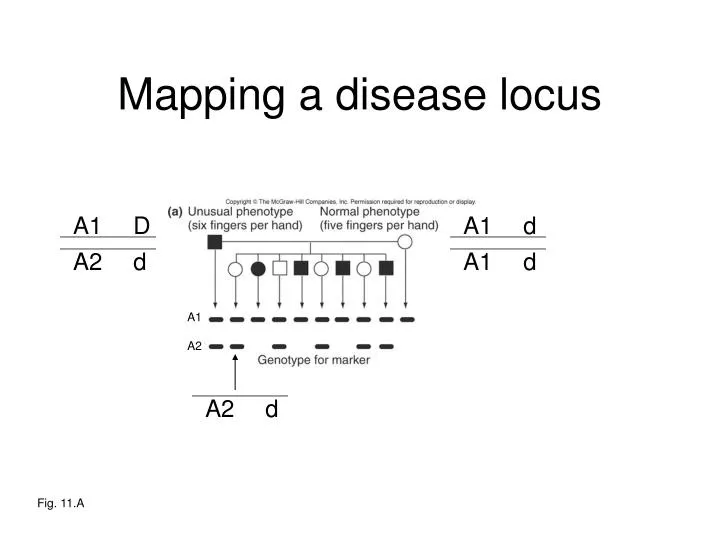
A1. d. A1. D. A1. d. A2. A2. d. d. Mapping a disease locus. A1 A2. Fig. 11.A. A1. d. A1. A1. D. D. A1. d. A2. d. Mapping a disease locus. A1 A2. Fig. 11.A. A1. d. A1. D. A1. d. A2. A2. D. d. Mapping a disease locus. (sperm). A1 A2. Fig. 11.A. LOD scores.

E N D
A1 d A1 D A1 d A2 A2 d d Mapping a disease locus A1 A2 Fig. 11.A
A1 d A1 A1 D D A1 d A2 d Mapping a disease locus A1 A2 Fig. 11.A
A1 d A1 D A1 d A2 A2 D d Mapping a disease locus (sperm) A1 A2 Fig. 11.A
LOD scores r = genetic distance between marker and disease locus Odds = P(pedigree | r) P(pedigree | r = 0.5) Odds = (1-r)n • rk 0.5(total # meioses) Data >6 times more likely under LINKED hypothesis than under UNLINKED hypothesis. Odds = 0.77 • 0.31 = 6.325 0.58 k = 1 recomb, n = 7 non-recomb. A1 A2
Just a point estimate True distance 30 cM Disease-causing mutation Restriction fragment length polymorphism observed recombination fraction = 1/8 = 12.5 cM this is our observation
LOD scores Odds = P(pedigree | r) k = 1 recomb, n = 7 non-recomb. P(pedigree | r = 0.5) Odds = (1-r)n • rk 0.5(total # meioses)
1,2 2,3 1,2 2,3 2,3 1,2 1,3 1,2 1,2 1,3 2,3 1,3 2,3 1,3 1,3 2,3 1,3 1,2 2,3 2,3 2,2 2,2 Combining families Given r Odds2 Given r Odds1 How to get an overall estimate of probability of linkage? Multiply odds together Add odds together Take the largest odds Take the average odds Given r Odds3
A1 d A1 A1 D d A1 d A2 A2 d D More realistic situation: in dad, phase of alleles unknown or A1 A2
A1 A1 D d A2 A2 D d More realistic situation: in dad, phase of alleles unknown P(pedigree|r) Odds = 1/2[(1-r)n • rk] + 1/2[(1-r)n • rk] assume one phase for dad assume the other phase for dad 7 non-recomb, 1 recomb 1 non-recomb, 7 recomb (k = # recomb, n = # non-recomb) A1 A2
In real life this correction does matter… family 1: 10 meioses, 1 (or 9) apparent recombinants family 2: 10 meioses, 4 (or 6) apparent recombinants family 3: 10 meioses, 3 (or 7) apparent recombinants family 4: 10 meioses, 3 (or 7) apparent recombinants total LOD = LOD(family 1) + LOD(family 2) + LOD(family 3) + LOD(family 4) Accounting for both phases Using only one phase best r = 0.2771 best r = 0.2873
Modern genetic scans (single family)
Age of onset in breast cancer age of onset
Coins r = intrinsic probability of coming up heads (bias) Odds = P(your flips | r) P(your flips | r = 0.5) Odds = (1-r)n • rk 0.5(total # flips)
Coins r = intrinsic probability of coming up heads (bias) 0 heads 1 heads 2 heads 3 heads 4 heads
Coins By chance, can get good LOD score for just about anything. The more students you have flipping coins, the more likely you are to see this “unlikely” combination. The multiple testing problem
Coins Probability of one student observing 0 heads and 4 tails: 1/16 Estimated number of students out of 70 observing 4 tails: 70*(1/16)= 4 Probability of one student observing 1 head and 3 tails: 4/16 Estimated number of students out of 70 observing 1 heads and 3 tails: 70*(4/16)= 17.5 Probability of one student observing 2 heads and 2 tails: 6/16 Estimated number of students out of 70 observing 2 heads and 2 tails: 70*(6/16) = 26.3 … We would need to see >4 students get 0 heads and 4 tails before we believe any coins are biased.
Simulation/theory Expect 0.09 of a locus to reach LOD=3 by chance.
Simulation/theory But this would change in a different organism, with different number of markers, etc. So in practice, everyone does their own simulation specific to their own study.
Candidate gene approach Hypothesize that causal variant will be in known pigment gene or regulator. NOT randomly chosen markers genome-wide.
Candidate gene approach Red progeny have RFLP pattern like red parent
Affected sib pair method … 2,2 2,3 4,4 1,3 Total # families 2,2 2,2 1,4 1,4 2 = (O - E)2 E Test for significant allele sharing.
Qualitative but polygenic Two loci. Need one dominant allele at each locus to get phenotype. Fig. 3.12
“A weak locus”: need lots of data AAbb aaBB inter-mate AaBb Two loci. Need one dominant allele at each locus to get phenotype. AaBb aaBB AABb aaBb AaBB Aabb Flower color Genotype at marker close to A locus
More generally (one locus): AA x BB AB (F1) AB x AB AA AB BA BB (F2)
1 locus, incomplete dominance AB BA “Effect of having a B” AA BB 25% 50% 25% AB BA AA BB Effect of a B allele is the same regardless of genotype: additive
1 locus, complete dominance ABBAAA BB 75% 25% Dominance is a kind of epistasis: nonadditive
A real example CC x SS CS (F2’s) CS x CS CC SS CS SC (F2’s)
Quantitative trait linkage test Not counting recombinants. Statistical test for goodness of fit. (F2’s)
Locus effect vs. parents Homozygotes do not look like parent. What do you infer? C3H parent F2’s, C/C at marker F2’s, C/S at marker F2’s, S/S at marker SWR parent A single varying locus does not explain the data
>1 locus controlling trait (One mouse family)
A weak locus “Effect of having an S allele” Most loci underlying human disease look like this. C3H parent F2’s, C/C at marker F2’s, C/S at marker F2’s, S/S at marker SWR parent
Heritability in exptal organisms e t Genetic variance = total var - “environmental var” Heritability H2 = g = t -e g/t
Heritability in humans: MZ twins http://www.sciam.com/media/inline/15DD5B0E-AB41-23B8-2B1E53E8573428C5_1.jpg http://www.twinsinsurance.net/images/twins.jpg http://www.twinsrealm.com/othrpics/twins16.jpg http://www.twinsrealm.com/othrpics/sarahandsandra.jpg Mean each pair = zi Each individual = zij b2 w2 (zij - z)2 h2 = Total mean sq = = t2 t2 T (zij - zi)2 Within pairs mean sq = = w2 N (zi - z)2 = b2 Between pairs mean sq = N-1
Linkage mapping (quantitative) intolerant tolerant
Fine-mapping: new markers Position of true causal variant Because you have to hunt through by hand to find the causal gene, and test experimentally. The smaller the region, the better. Best marker
Fine-mapping: new markers Position of true causal variant Increased marker density
Two loci, incomplete dominance 0.5 1 1.5 2
2-locus interaction Effect of J at locus 2 Locus 2 is epistatic to locus 1: effects of locus 1 are masked in individuals with JJ or JL,LJ at locus 2 Locus 2 follows a dominance model: JJ and JL,LJ have the same phenotype, LL differs “The dominant allele of locus 2 does the masking”
Three mutant genes From pathogenic strain From pathogenic strain From pathogenic strain Alleles from the same strain at different genes/loci can have different effects.
Linked mutations of opposite effect Path Lab Very unlikely
Fine-mapping WT uninjected Golden uninjected Inject into golden larvae
No truncation in humans, but… No other species have the Thr allele: what does this mean? Could be deleterious, just an accidental mutation. Could be advantageous for some humans, no other species.
Correlates with human differences Allele is rare AA Thr AG Thr, Ala Perhaps explains phenotypic variation among people of African ancestry GG Ala
Association mapping (qualitative) Blue alleles at markers are on the same haplotype as the M allele of the disease locus Fig. 11.26
Association scan, qualitative 2 test
Fine-mapping -log(2p-value) rs377472
Beginnings of molecular confirmation coding polymorphisms