Download

1 / 34
340 likes | 342 Views
Learn how changes in the price level affect the aggregate demand and supply. Understand the concept of macroeconomic equilibrium and how shocks impact real GDP and price levels.

E N D
* Chapter 23 Output and Prices in the Short Run
In this chapter you will learn 1. why an exogenous change in the price level shifts the AE curve and changes the equilibrium level of real GDP. 2. how to derive the aggregate demand (AD) curve and what causes it to shift. 3. the meaning of the aggregate supply (AS) curve and why it shifts when technology or factor prices change.
In this chapter you will learn 4. how to define macroeconomic equilibrium. 5. how aggregate demand and aggregate supply shocks affect real GDP and the price level.
* 23.1 THE DEMAND SIDE OF THE ECONOMY Exogenous Changes in the Price Level – what are they? Exogenous means ‘from outside the system’ – something not explained in our model (eg. G, interest rates, exchange rates, the weather) Endogenous means ‘from within our system’ – something explained in our model (eg. Y, AE, C, M) MFC2007MFC2007,MFC2007,MFC2007MFC2007MFC2007
What do we mean by an exogenous increase or decrease in prices ? The Canadian price level (P) increases for some reason not explained as part of our macroeconomic story. Example - natural resource prices in world markets increase causing Canadian natural resources prices to rise and this feeds through to production costs and ultimately P (the general price level). Or - a new Gov’t safety regulation causes all prices to go up. MFC2007MFC2007,MFC2007,MFC2007MFC2007MFC2007
* Exogenous Changes in the Price Level – why do they matter? An increase in P reduces the real value of money holdings. A fall in P raises the real value of money holdings. Changes in P affect the wealth of both private bondholders and private bond issuers - but there is no change in aggregate wealth of the private sector. BUT What about government debt? - Changes in P make the Gov’t debt worth less – this does affect the wealth of the private sector MFC2007MFC2007,MFC2007,MFC2007MFC2007MFC2007
An increase in P thus reducesprivate-sector wealth: - causing a reduction in desired consumption - resulting in a downward shift in AE curve There is also an effect on net exports (recall relative prices in Canada in in foreign countries): - the NX function shifts downward and steepens - resulting in a further downward shift in AE curve The opposite happens for a fall in P. MFC2007MFC2007,MFC2007,MFC2007MFC2007MFC2007
* Changes in Equilibrium GDP An increase in P reduces desired aggregate expenditure (C and NX shift downward): - AEshifts down - equilibrium Y falls AE AE =Y AE0 (P0) E0 • AE1 (P1) • E1 Y1 Y0 Y where P1 > P0 MFC2007MFC2007,MFC2007,MFC2007MFC2007MFC2007
* Changes in Equilibrium GDP A decrease in P increases desired aggregate expenditure (C and NX shift upwards): - AEshifts up - equilibrium Y increase AE AE =Y AE1 (P1) E1 • AE0 (P0) • E0 Y0 Y1 Y where P1 < P0 MFC2007MFC2007,MFC2007,MFC2007MFC2007MFC2007
The Aggregate Demand Curve The aggregate demand (AD) curve relates equilibrium real GDP (Y) to the price level. For any given P, the AD curve shows the level of real GDP (Y) for which desired aggregate expenditure equals actual GDP (Y). Changes in the price level cause movements along the AD curve.
AE =Y AE * E0 AE0 ( at P0) • AE1 (at P1 > P0) E1 AE2 (at P2 > P1) • Consider a rise in the price level, from P0 to P2: E2 • Y2 Y1 Y0 Y P The AE curve shifts down as P rises, but we move along the AD curve. • P2 P1 • P0 • AD Y2 Y1 Y0 Y MFC2007MFC2007,MFC2007,MFC2007MFC2007MFC2007
AE =Y AE Shifts in the AD Curve when P is constant * AE1 (P0) E1 • AE0 (P0) Any shock that increases equilibrium GDP at a given price level shifts the AD curve to the right. Recall - interest rates - wealth (non P related) - confidence (expectations) - foreign incomes - exchange rates - change in G - etc. E0 • Y0 Y1 Y P E1 E0 P0 • • AD1 The horizontal shift of the AD curve is the simple multiplier times the change in autonomous spending. AD0 Y0 Y1 Y MFC2007MFC2007,MFC2007,MFC2007MFC2007MFC2007
23.2 THE SUPPLY SIDE OF THE ECONOMY The Aggregate Supply Curve The AS curve relates the price level to the quantity of output that firms would like to produce and sell. The AS curve is drawn for a given - level of technology - set of factor prices. Since unit costs (Marginal Costs) rise with output, firms will produce more output only if prices increase. AS curve is upward sloping
What does the Aggregate Supply Curve look like? Until this point we have assumed that the aggregate supply (AS) was perfectly elastic (a horizontal straight line) Why? Firms had plenty of unused capacity, unemployed workers and resources. Firms could expand production without incurring rising marginal costs. Firms would produce any level of output demanded at the existing price level. Price Level AS0 P0 • • This is a purely Keynesian type assumption. Is it true today? Maybe in some industries. Y1 Y0 Y (GDP) MFC2007MFC2007,MFC2007,MFC2007MFC2007MFC2007
What does the Aggregate Supply Curve look like? Because unit costs rise with output (Marginal Costs generally increases as output increases) firms will produce more output only if prices increase. The AS curve is therefore upward sloping. Price Level This is straight out of the microeconomics of the firm. In the short run firms generally find that MC increases as output increases so they will increase production only if they get higher prices. AS1 P1 • P0 • Y0 Y1 Y (GDP) MFC2007MFC2007,MFC2007,MFC2007MFC2007MFC2007
What does the Aggregate Supply Curve look like? The slope of the AS curve is relatively flat when output is low, firms typically have excess capacity (Keynesian section). This means that output can be expanded without causing a significant increase in unit costs. Price Level AS1 But as more and more capacity is used the marginal cost of producing additional units of output goes up faster and faster and the AS curve gets steeper. • P1 P0 • Y1 Y0 Y (GDP) MFC2007MFC2007,MFC2007,MFC2007MFC2007MFC2007
Shifts in the Aggregate Supply Curve Anything that increases firms’ costs causes the AS curve to shift up: - increases in factor prices - reversal in technology - increased regulation - weather, etc. Price Level AS1 AS0 P1 • P0 • • Y0 Y1 Y (GDP) MFC2007MFC2007,MFC2007,MFC2007MFC2007MFC2007
* Shifts in the Aggregate Supply Curve Anything that decreases firms’ costs causes the AS curve to shift down: - decrease in factor prices - improved technology - less regulation - weather, etc. Price Level AS0 AS1 P0 • P1 • • Y1 Y0 Y (GDP) MFC2007MFC2007,MFC2007,MFC2007MFC2007MFC2007
The slope of the AS curve is increasing as output rises: - when output is low, firms typically have excess capacity costs do not rise quickly - when output is nearer Y*, costs rise as output rises firms need higher prices EXTENSIONS IN THEORY 23-1 The Keynesian AS Curve
* 23.3 MACROECONOMIC EQUILIBRIUM Aggregate Demand (AD) - what consumers, investors, governments and foreigners want to buy from Canadian firms at a given P Aggregate Supply (AS) - what Canadian firms want to sell at a given P AD is equal to AS only at the intersection of the two curves. AD Price Level AS E0 P0 • Y0 E0 is the macroeconomic equilibrium. Y (GDP) MFC2007MFC2007,MFC2007,MFC2007MFC2007MFC2007
* Demand behaviour is only consistent with supply behaviour at the intersection of the AS and AD curves. AD AS Price Level At P1 there is more output demanded (Y2) than what firms want to produce (Y1). E0 P0 • P1 • • Therefore prices will rise and output will increase until the excess aggregate demand is eliminated. Y2 Y0 Y1 Y (GDP) MFC2007MFC2007,MFC2007,MFC2007MFC2007MFC2007
* At P2 there is less output demanded (Y1) than what firms want to produce (Y2). AD AS Price Level Therefore prices will fall and output will decrease until the excess aggregate supply is eliminated. P2 • • E0 P0 • Y2 Y0 Y1 Y (GDP) MFC2007MFC2007,MFC2007,MFC2007MFC2007MFC2007
Changes in the Macroeconomic Equilibrium Demand shocks can either be expansionary or contractionary - direction of AD shift AD shifts out - expansionary AD shifts in - contractionary Supply shocks can either be expansionary or contractionary - direction of the AS shift AS shifts out - expansionary AS shifts in - contractionary In both cases, “expansionary” or “contractionary” refers to the effect on equilibrium output. MFC2007MFC2007,MFC2007,MFC2007MFC2007MFC2007
* Aggregate Demand Shocks – Positive shock Demand shocks cause P and Y to change in the same direction. Possible causes: - ΔG > 0 - ΔI > 0 eg. r - ΔX > 0 eg. exchange rate - ΔC > 0 eg. confidence Price Level AD1 AS AD0 P1 • E1 E0 P0 • Y0 Y1 Y (GDP) P increases and Y increases MFC2007MFC2007,MFC2007,MFC2007MFC2007MFC2007
* Aggregate Demand Shocks- Negative shock Demand shocks cause P and Y to change in the same direction. Possible causes: - ΔG < 0 - ΔI < 0 eg. r - ΔX < 0 eg. exchange rate - ΔC < 0 eg. confidence Price Level AD0 AS AD1 P0 • E0 E1 P1 • Y1 Y0 Y (GDP) P decreases and Y decreases MFC2007MFC2007,MFC2007,MFC2007MFC2007MFC2007
If the AS curve is flat, then firms are willing to produce more output at current prices (Chapter 21 and 22). We get the simple multiplier effect. But with an upward sloping AS curve, the multiplier is smaller than the simple multiplier. WHY? Because firms are operating in the rising portion of their Marginal Cost Curve – costs are rising with additional output. P AS2 E2 AS1 P2 • E1 P0 • • E0 AD1 AD0 Y Y0 Y2 Y1 MFC2007MFC2007,MFC2007,MFC2007MFC2007MFC2007
AD5 * AD4 AS AD3 P5 The effect of any given shift of the AD curve will depend on the slope of the AS curve. AD2 P4 AD1 • Price Level AD0 P3 • P2 • P0 • • The steeper the AS curve, the greater the price effect and the smaller the output effect. Y0 Y1 Y2 Y3 Y4 Y (GDP)
* Aggregate Supply Shocks - Positive shock Aggregate supply shocks cause P and Y to change in opposite directions. Possible causes: - decrease price of non- wage inputs - decrease in wages - improvement in technology - decreased regulation P AS0 AS1 E0 P0 • E1 P1 • P decreases and Y increases NICE! AD Y0 Y1 MFC2007MFC2007,MFC2007,MFC2007MFC2007MFC2007
* Aggregate Supply Shocks - Negative shock Aggregate supply shocks cause P and Y to change in opposite directions. Possible causes: - increase price of non- wage inputs - increase in wages - reversal in technology - increased regulation P AS1 AS0 E1 P1 • E0 P0 • P increases and Y decreases OUCH! AD Y1 Y0 MFC2007MFC2007,MFC2007,MFC2007MFC2007MFC2007
* Offsetting changes in wages and productivity If wage rise at the same rate as productivity increases then there is no net effect An increase in wages causes a negative supply shock An increase in productivity causes a positive supply shock AS’0 P Negative supply shock if wages rise faster than productivity Positive supply shock if wages rise more slowly than productivity AS0 E0 P0 • AD Y0 MFC2007MFC2007,MFC2007,MFC2007MFC2007MFC2007
A Word of Warning Many economic events (especially changes in the world prices of raw materials) cause both aggregate demand and aggregate supply shocks. The overall effect on the economy depends on the relative importance of the two separate effects. LESSONS FROM HISTORY 23-1 The Asian Crisis and the Canadian Economy
* The Canadian Economy is being ‘shocked’ all the time. Many of these AD and AS shocks are relatively small and cancel out. To make real world predictions about the future level of P and Y we would need to keep track of many possible changes (G, r, exchange rates, confidence levels, input prices, technology, etc., etc.) Consider an increase in energy prices which Increase costs to firms and the wealth of Canadians Y Y1 Y0 P AS1 AS0 The overall outcome for the economy depends on the relative importance of the two separate effects. P1 E1 AD1 • E0 P0 • AD0 Y0 Y1 MFC2007MFC2007,MFC2007,MFC2007MFC2007MFC2007
The increase in the world price of oil from 2002 to 2006 was dramatic, but many observers were surprised at its modest impact on the Canadian economy. For more information on how changes in oil prices affect Canada, and for why the negative ASeffect is smaller now than in the 1970s, look for “Oil Prices and the Canadian Economy” in the Additional Topics section of this book’s MyEconLab. www.myeconlab.com