Download
1 / 36
390 likes | 1k Views
Analysis of Variance for Some Fixed-, Random-, and Mixed-Effects Models. Chapter 17. Definition 17.1.

E N D
Analysis of Variance for Some Fixed-, Random-, and Mixed-Effects Models Chapter 17
Definition 17.1 In a fixed-effects model for an experiment, all the factors in the experiment have a predetermined set of levels and the only inferences are for the levels of the factors actually used in the experiment.
Definition 17.2 In a random effects model for an experiment, the levels of factors used in the experiment are randomly selected from a population of possible levels. The inferences from the data in the experiment are for all levels of the factors in the population from which the levels were selected and not only the levels used in the experiment.
Definition 17.3 In a mixed-effects model for an experiment, the levels of some of the factors used in the experiment are randomly selected from a population of possible levels, whereas the levels of the other factors in the experiment are predetermined. The inferences from the data in the experiment concerning factors with fixed levels are only for the levels of the factors used in the experiment, whereas inferences concerning factors with randomly selected levels are for all levels of the factors in the population from which the levels were selected.
Designing the Data Collection • Which factors should be used in the study? • Which levels of the factors are of interest? • How many levels are needed to adequately identify the important sources of variation? • How many replications per factor-level combinations are needed to obtain a reliable estimate of the variance components?
Designing the Data Collection, cont. • What environmental factors may affect the performance of the pressure gauge during the test period? • What are the valid statistical procedures for evaluating the causes of the variability in pressure drops across the expansion joints? • What type of information should be included in a final report to document that all important sources of variability have been identified?
The Model • Fixed-effects model • Random-effects model: the terms are the same but some of the assumptions are different • is still the overall mean, which is an unknown constant. • i is a random effect due to the ith tracking station. We assume that i is normally distributed, with mean 0 and variance .
The Model, cont. • The i‘s are independent. • As before, ij is normally distributed, with mean 0 and variance . • The ij ‘s are independent. • The random components i andij are independent.
Table 17.2: An AOV table for a one-factor experiment: fixed or random model
Observations • Note in Table 17.2 that the AOV table is the same for both the fixed- and random-effects model, however the expected mean squares (EMS) are different. • In general, with t treatments and r observations/treatment, the AOV table would appear as in table 17.2 • For the fixed-effects model, we would test for equality of means of the treatments.
Observations, cont. • For the random-effects model, we would test for variability in the population of treatment values.
Table 17.3: Proportional allocation of total variability in the response variable
Extending the Random-Effects Model to a Randomized Block Design • The Model: • Assumptions: • is an overall unknown mean of the response • i is a random effect due to the ith treatment. i is normally distributed, with mean 0 and variance . • The i s are independent.
Extending the Random-Effects Model to a Randomized Block Design, cont. • Assumptions cont. : • j is a random effect due to the jth block. j is a normally distributed random variable, with mean 0 and variance . • The j s are independent. • The i s, j s, and ij s are independent.
Table 17.7: AOV table for a two-factor experiment, a Levels of factor A and b Levels of factor B
The Random Effects Model for an ab Factorial Experiment • Model: • Assumptions: • ijis a random effect due to the ith level of factor A and the jth level of factor B. ij is normally distributed, with mean 0 and variance . • The ijs are independent. • The is, js, ijs, and ijks are independent.
Table 17.9: AOV table for an a b factorial experiment, with nobservations per cell
Table 17.10: A comparison of appropriate interaction tests for fixed- and random-effects models
Table 17.11: Tests for an a b factorial experiment with replication: random-effects model
Table 17.12: Proportional allocation of total variability in the response variable
Mixed-Effects Models • Suppose we have the levels of factor A fixed and the levels of factor B randomly selected. • Model: • Assumptions: • is the unknown overall mean response. • iis a fixed effect corresponding to the ith level of factor A
Mixed-Effects Models, cont. • Assumptions, cont.: • jis a random effect due to the jth level of factor B. The js have independent normal distributions, with mean 0 and variance . • ijis a random effect due to the interaction of the ith level of factor A with the jth level of factor B . The ijs have normal distributions with mean 0 and variance . For all j j , ij and i j are independent. • The js, ijs, and ijks are independent.
Mixed-Effects Models, cont. Test for :
Table 17.13: AOV table for an a b factorial experiment, with n observations per cell
Rules for Obtaining Expected Mean Squares • Let SPSS DO IT
1 2 1 1 2 2 3 3 Figure 17.2: Two-factor experiment with batches nested in sites Sites Batches in sites Samples in batches 1 2 3…10 1 2 3…10 1 2 3…10 1 2 3…10 1 2 3…10 1 2 3…10
The Model • Two factor experiment with factor B nested in factor A
Table 17.29: AOV table for a two-factor experiment (n observations per cell) with factor B nested in factor A
2 3 4 1 T1 T2 T3 T3 T1 T2 T3 T1 T1 T2 T2 T3 Figure 17.3: Split-Plot Design A1 A2 A3 A4 Wholeplot Wholeplot Wholeplot Wholeplot
Figure 17.4: Two-stage randomization for a completely randomized split-plot design Wholeplot 2 3 4 1 A1 A2 A2 A1 (a) Wholeplot 2 3 4 1 T1 T2 T3 T3 T1 T2 T3 T1 T1 T2 T2 T3 (b)
The Model where i: Fixed effect for ith level of A τj: Fixed effect for jth level of T τij : Fixed effect for ith level of A, jth level of T
The Model, cont. ik: Random effect for the kth wholeplot receiving the ith level of A. The ik are independent normal with mean 0 and variance . ijk: Random error. The ijk are independent normal with mean 0 and variance . The ik and ijk are mutually independent.
Figure 17.5: Randomized block split-plot design Blocks 2 1 T2 T1 T3 T1 T3 T2 T3 T1 T2 T3 T2 T1 A2 A2 A1 A1 The Model: