Advanced Computer Vision Chapter 11 Stereo Correspondence

1. Advanced Computer VisionChapter 11 Stereo Correspondence Presented by: 蘇唯誠 0921679513 r02922114@ntu.edu.tw 指導教授: 傅楸善 博士

2. Introduction • Stereo matching is the process of taking two or more images and estimating a 3D model of the scene by finding matching pixels in the images and converting their 2D positions into 3D depths. • In this chapter, we address the question of how to build a more complete 3D model.

3. (a) (b) (c) (d) (e) (f)

4. 11.1 EpipolarGeometry • Given a pixel in one image, how can we compute its correspondence in the other image? • We exploit this information to reduce the number of potential correspondences, and hence both speed up the matching and increase its reliability.

5. (Faugerasand Luong 2001; Hartley and Zisserman 2004).

6. 11.1.1 Rectification • We can use the epipolar line corresponding to a pixel in one image to constrain the search for corresponding pixels in the other image. • One way to do this is to use a general correspondence algorithm, such as optical flow. • A more efficient algorithm can be obtained by first rectifying (i.e, warping).

7. (a) (b) (c) (d) (a) Original image pair overlaid with several epipolar lines; (b) images transformed so that epipolar lines are parallel; (c) images rectified so that epipolar lines are horizontal and in vertial correspondence; (d) final rectification that minimizes horizontal distortions. (Loop and Zhang 1999; Faugerasand Luong 2001; Hartley and Zisserman 2004).

8. 11.1.1 Rectification • The epipolar constrain is defined for all pairs of images correspondences and , where is so-called fundamental matrix. • For a fundamental matrix there exists a pair of unique points and such that .

9. 11.1.1 Rectification • Image rectification can be view as the process of transforming the epipolar geometry of a pair of images into a canonical form. • This is accomplished by applying a homography to each image that maps the epipole to a predetermined point , and the fundamental matrix for a rectified image pair is defined • Where is the antisymetric matrix representing the cross product with .

10. 11.1.1 Rectification • Rectified images have the following two properties: • All epipolar lines are parallel to the u-coordinate axis • Corresponding points have identical v-coordinates

11. 11.1.1 Rectification • Let and be the homographies to be applied to images and respectively. • and • The homographiesand are not unique. • Our task is to find a pair of homographiesand minimize image distortion.

12. 11.1.1 Rectification • Let , , and be lines equated to the rows of such that

13. 11.1.1 Rectification • Decomposition of the homographies • Dividing out from • Compute • Where is a projective transform, is similarity transform, and is shearing transform.

14. (a) (b) (c) (d) (a) Original image pair overlaid with several epipolar lines; (b) images transformed so that epipolar lines are parallel; (c) images rectified so that epipolar lines are horizontal and in vertial correspondence; (d) final rectification that minimizes horizontal distortions. (Loop and Zhang 1999; Faugerasand Luong 2001; Hartley and Zisserman 2004).

15. 11.1.1 Rectification • The resulting standard rectified geometry is employed in a lot of stereo camera setups and stereo algorithms, and leads to a very simple inverse relationship between 3D depths Zand disparities d, • where f is the focal length (measured in pixels), B is the baseline, and

16. 11.1.1 Rectification • The task of extracting depth from a set of images then becomes one of estimating the disparity map d(x, y). • After rectification, we can easily compare the similarity of pixels at corresponding locations (x, y) and (x0, y0) = (x + d, y) and store them in a disparity space image C(x, y, d) for further processing. • DSI: disparity space image

18. Bobickand Intille(1999).

19. 11.2 Sparse correspondence • Early stereo matching algorithms were feature-based, i.e., they first extracted a set of potentially matchableimage locations, using either interest operators or edge detectors, and then searched for corresponding locations in other images using a patch-based metric. (Hannah 1974; Marr and Poggio 1979; Mayhew and Frisby 1980; Baker and Binford 1981; Arnold 1983; Grimson 1985; Ohta and Kanade 1985; Bolles, Baker, and Marimont 1987; Matthies, Kanade, and Szeliski 1989; Hsieh, McKeown, and Perlant 1992; Bolles, Baker, and Hannah 1993).

20. 11.2.1 3D curves and profiles • Another example of sparse correspondence is the matching of profile curves. • Let us assume that the camera is moving smoothly enough that the local epipolargeometry varies slowly.

21. (a) (b) (c) (d) (e) (f) (g) (a) circular arc fitting in the epipolar plane; (b) synthetic example of an ellipsoid with a truncated side and elliptic surface markings; (c) partially reconstructed surface mesh seen from an oblique and top-down view; (d) real-world image sequence of a soda can on a turntable; (e) extracted edges; (f) partially reconstructed profile curves; (g) partially reconstructed surface mesh.

22. 11.2.1 3D curves and profiles • If we parameterize the osculating circle by its center and radius , we find that the tangency condition between line and the circle can be written as

23. 11.2.1 3D curves and profiles • where , , and • , where is the camera center and normalizes a vector. • , where is the normal vector of epipolar plane.

25. 11.3 Dense correspondence • While sparse matching algorithms are still occasionally used, most stereo matching algorithms today focus on dense correspondence, since this is required for applications such as image-based rendering or modeling. • This problem is more challenging than sparse correspondence.

26. 11.3 Dense correspondence (cont’) • It is based on the observation that stereo algorithms generally perform some subset of the following four steps: • 1. matching cost computation; • 2. cost (support) aggregation; • 3. disparity computation and optimization; and • 4. disparity refinement.

27. 11.3 Dense correspondence (cont’) • For example, the traditional sum-of-squared differences (SSD) algorithm can be described as: • 1. The matching cost is the squared difference of intensity values at a given disparity. • 2. Aggregation is done by summing the matching cost over square windows with constant disparity. • 3. Disparities are computed by selecting the minimal (winning) aggregated value at each pixel.

28. 11.3 Dense correspondence (cont’) • Global algorithms, on the other hand, make explicit smoothness assumptions and then solve a global optimization problem (Section 11.5). • Such algorithms typically do not perform an aggregation step, but rather seek a disparity assignment (step 3) that minimizes a global cost function that consists of data (step 1) terms and smoothness terms.

29. 11.4 Local methods • Local and window-based methods aggregate the matching cost by summing or averaging over a support region in the DSI C(x, y, d). • DSI: Disparity Space Image • Aggregation has been implemented using square windows or Gaussian convolution (traditional).

30. 11.5 Global optimization • Global stereo matching methods perform some optimization or iteration steps after the disparity computation phase and often skip the aggregation step altogether. • Many global methods are formulated in an energy-minimization framework.

31. 11.5 Global optimization (cont’) • The objective is to find a solution d that minimizes a global energy, • The data term, Ed(d), measures how well the disparity function d agrees with the input image pair. • where C is the (initial or aggregated) matching cost DSI.

32. 11.5 Global optimization (cont’) • The smoothness term is often restricted to measuring only the differences between neighboring pixels’ disparities, • where ᵨis some monotonically increasing function of disparity difference.

33. 11.6 Multi-view stereo • While matching pairs of images is a useful way of obtaining depth information, matching more images can lead to even better results.

34. 11.6 Multi-view stereo

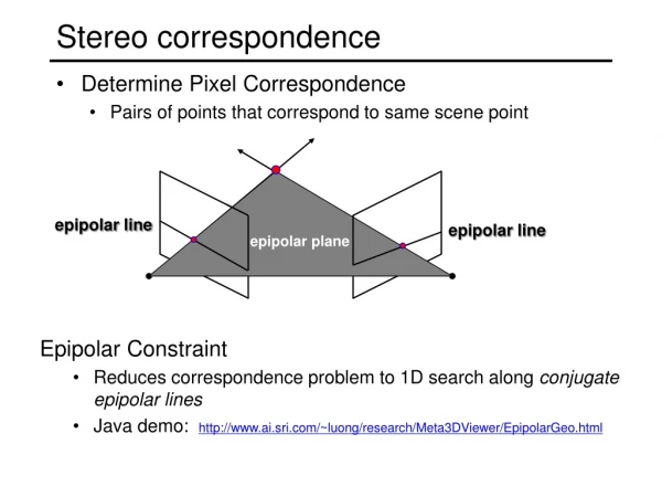
35. Automated Stereo Perception • Following introduces the subproblem of one-dimensional stereo matching. • Consider a pair of corresponding epipolar lines from a stereo image pair.

37. Automated Stereo Perception • Rays from the left and right cameras intersect to from a grid or lattice. • This lattice is bounded by a region obtained by projecting rays through the image boundaries. • We will refer to this region as the stereo zone, for only objects within this zone can be seen in stereo.

38. Automated Stereo Perception

39. Automated Stereo Perception • Each lattice point corresponds to a potential match between a feature in the left and a feature in the right. • If such a match were correct, then the object must have been at the point space represented by that lattice point.

40. Automated Stereo Perception • We have six types of profile intervals: • The surface and both edges are visible to both cameras. • The surface and its left edge are visible to both cameras, but its right edge is occluded. • The surface is visible only to the left camera. • The surface is visible only to the right camera. • The surface and its right edge are visible to both cameras, but its left edge is occluded. • The surface is visible to both cameras, but its left and right edges are occluded.

41. Automated Stereo Perception

43. Automated Stereo Perception • Summary: • This section introduced some basic stereo matching. • We describe the geometry and develop a notation for a stereo system.

44. END