Download
1 / 22
230 likes | 444 Views
Modeling uncertainty propagation in deformation processes. Babak Kouchmeshky Nicholas Zabaras. Materials Process Design and Control Laboratory Sibley School of Mechanical and Aerospace Engineering 101 Frank H. T. Rhodes Hall Cornell University Ithaca, NY 14853-3801

E N D
Modeling uncertainty propagation in deformation processes Babak Kouchmeshky Nicholas Zabaras Materials Process Design and Control Laboratory Sibley School of Mechanical and Aerospace Engineering101 Frank H. T. Rhodes Hall Cornell University Ithaca, NY 14853-3801 URL: http://mpdc.mae.cornell.edu/ Materials Process Design and Control Laboratory
Problem definition • Obtain the variability of macro-scale properties due to multiple sources of uncertainty in absence of sufficient information that can completely characterizes them. • Sources of uncertainty: • - Process parameters • - Micro-structural texture Materials Process Design and Control Laboratory
The coefficients correspond to tension/compression,plain strain compression, shear and rotation. Sources of uncertainty (process parameters) Since incompressibility is assumed only eight components of L are independent. Materials Process Design and Control Laboratory
Sources of uncertainty (Micro-structural texture) Continuum representation of texture in Rodrigues space Underlying Microstructure Fundamental part of Rodrigues space Variation of final micro-structure due to various sources of uncertainty Materials Process Design and Control Laboratory
Variation of macro-scale properties due to multiple sources of uncertainty on different scales use Frank-Rodrigues space for continuous representation Uncertain initial microstructure Use Karhunen-Loeve expansion to reduce this random filed to few random variables Considering the limited information Maximum Entropy principle should be used to obtain pdf for these random variables Use Rosenblatt transformation to map these random variables to hypercube Use Stochastic collocation to obtain the effect of these random initial texture on final macro-scale properties. Limited snap shots of a random field Materials Process Design and Control Laboratory
Evolution of texture ORIENTATION DISTRIBUTION FUNCTION – A(s,t) • Determines the volume fraction of crystals within • a region R' of the fundamental region R • Probability of finding a crystal orientation within • a region R' of the fundamental region • Characterizes texture evolution ODFEVOLUTION EQUATION – LAGRANGIAN DESCRIPTION Any macroscale property < χ > can be expressed as an expectation value if the corresponding single crystal property χ (r ,t) is known. Materials Process Design and Control Laboratory
Constitutive theory F F F B B o p * D = Macroscopic stretch = Schmid tensor = Lattice spin W = Macroscopic spin = Lattice spin vector (1) State evolves for each crystal (2) Ability to capture material properties in terms of the crystal properties Polycrystal plasticity Velocity gradient Deformed configuration Initial configuration s0 s n n0 Symmetric and spin components s0 n0 Stress free (relaxed) configuration Reorientation velocity Divergence of reorientation velocity Materials Process Design and Control Laboratory
Let be a second-order stochastic process defined on a closed spatial domain D and a closed time interval T. If are row vectors representing realizations of then the unbiased estimate of the covariance matrix is where and are eigenvalues and eigenvectors of and is a set of uncorrelated random variables whose distribution depends on the type of stochastic process. Representing the uncertain micro-structure Karhunen-Loeve Expansion: Then its KLE approximation is defined as Materials Process Design and Control Laboratory
Karhunen-Loeve Expansion Realization of random variables can be obtained by where denotes the scalar product in . The random variables have the following two properties Materials Process Design and Control Laboratory
Obtaining the probability distribution of the random variables using limited information • In absence of enough information, Maximum Entropy principle is used to obtain the probability distribution of random variables. • Maximize the entropy of information considering the available information as set of constraints Materials Process Design and Control Laboratory
Maximum Entropy Principle Constraints at the final iteration Materials Process Design and Control Laboratory
Inverse Rosenblatt transformation • Inverse Rosenblatt transformation has been used to map these random variables to 3 independent identically distributed uniform random variables in a hypercube [0,1]^3. • Adaptive sparse collocation of this hypercube is used to propagate the uncertainty through material processing incorporating the polycrystal plasticity. Materials Process Design and Control Laboratory
STOCHASTIC COLLOCATION STRATEGY Since the Karhunen-Loeve approximation reduces the infinite size of stochastic domain representing the initial texture to a small space one can reformulate the SPDE in terms of these N ‘stochastic variables’ Use Adaptive Sparse Grid Collocation (ASGC) to construct the complete stochastic solution by sampling the stochastic space at M distinct points • Two issues with constructing accurate interpolating functions: • What is the choice of optimal points to sample at? • 2) How can one construct multidimensional polynomial functions? • X. Ma, N. Zabaras, A stabilized stochastic finite element second order projection methodology for modeling natural convection in random porous media, JCP • D. Xiu and G. Karniadakis, The Wiener-Askey polynomial chaos for stochastic differential equations, SIAM J. Sci. Comp. 24 (2002) 619-644 • X. Wan and G.E. Karniadakis, Beyond Wiener-Askey expansions: Handling arbitrary PDFs, SIAM J Sci Comp 28(3) (2006) 455-464 Materials Process Design and Control Laboratory
Numerical Examples where are uniformly distributed random variables between 0.2 and 0.6 (1/sec). Example 1 : The effect of uncertainty in process parameters on macro-scale material properties for FCC copper A sequence of modes is considered in which a simple compression mode is followed by a shear mode hence the velocity gradient is considered as: Number of random variables: 2 Materials Process Design and Control Laboratory
Numerical Examples (Example 1) Adaptive Sparse grid (level 8) 1.28e05 4.02e07 1.28e05 3.92e07 MC (10000 runs) Materials Process Design and Control Laboratory
Numerical Examples (Example 2) Example 2 : The effect of uncertainty in process parameter (forging velocity ) on macro-scale material properties in a closed die forming problem for FCC copper Number of random variables: 1 Materials Process Design and Control Laboratory
Numerical Examples (Example 2) Materials Process Design and Control Laboratory
Numerical Examples (Example 3) Example 3 : The effect of uncertainty in initial texture on macro-scale material properties for FCC copper A simple compression mode is assumed with an initial texture represented by a random field A The random field is approximated by Karhunen-Loeve approximation and truncated after three terms. The correlation matrix has been obtained from 500 samples. The samples are obtained from final texture of a point simulator subjected to a sequence of deformation modes with two random parameters uniformly distributed between 0.2 and 0.6 sec^-1 (example1) Materials Process Design and Control Laboratory
Numerical Examples (Example 3) Step1. Reduce the random field to a set of random variables (KL expansion) Materials Process Design and Control Laboratory
Numerical Examples (Example 3) Step2. In absence of sufficient information,use Maximum Entropy to obtain the joint probability of these random variables Enforce positiveness of texture Materials Process Design and Control Laboratory
Numerical Examples (Example 3) Step3. Map the random variables to independent identically distributed uniform random variables on a hypercube [0 1]^3 are needed. The last one is obtained from the MaxEnt problem and the first 2 can be obtained by MC for integrating in the convex hull D. Rosenblatt transformation Rosenblatt M, Remarks on multivariate transformation, Ann. Math. Statist.,1952;23:470-472 Materials Process Design and Control Laboratory
Numerical Examples (Example 3) Adaptive Sparse grid (level 8) 1.41e05 4.42e08 MC 10,000 runs 4.39e08 1.41e05 Step4. Use sparse grid collocation to obtain the stochastic characteristic of macro scale properties Mean of A at the end of deformation process Variance of A at the end of deformation process FCC copper Variation of stress-strain response Materials Process Design and Control Laboratory