Download
1 / 89
920 likes | 937 Views
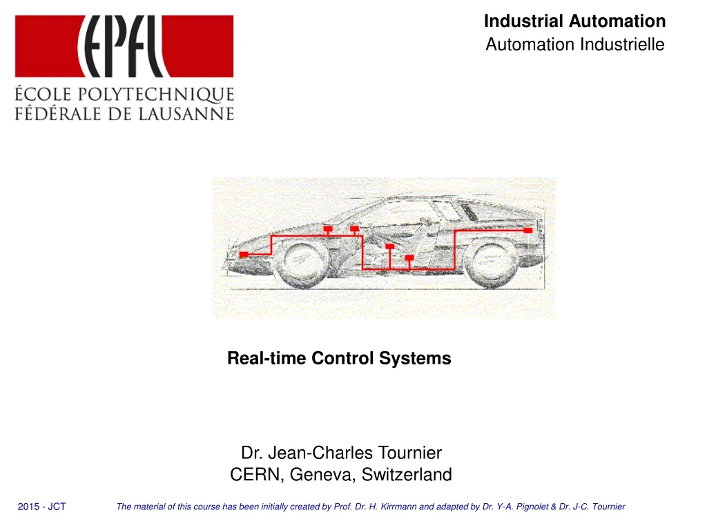
Industrial Automation Automation Industrielle. Real-time Control Systems. Dr. Jean-Charles Tournier. CERN, Geneva, Switzerland. 2015 - JCT. The material of this course has been initially created by Prof. Dr. H. Kirrmann and adapted by Dr. Y-A. Pignolet & Dr. J-C. Tournier. Enterprise

E N D
Industrial AutomationAutomation Industrielle Real-time Control Systems Dr. Jean-Charles Tournier CERN, Geneva, Switzerland 2015 - JCT The material of this course has been initially created by Prof. Dr. H. Kirrmann and adapted by Dr. Y-A. Pignolet & Dr. J-C. Tournier
Enterprise Applications • Real Time Industrial System • Resource planning • Maintenance • Cyclic • Condition-based • Planning & Forecasting • SCADA • Alarm management (EEMU 191) • Real-Time Databases • Domain Specific Applications • EMS/DMS • Outage management • GIS connections Supervision • HART • MMS • OPC Device Access • Time Synchronization • PPS, GPS, SNTP, PTP, etc. • Traditional - Modbus, CAN, etc. • Ethernet-based - HSR, WhiteRabbit, etc. Real-Time Field Buses Reliability • PLC • SoftPLC • PID PLCs/IEDs • Instrumentation • 4-20 mA loop • Sensors accuracy • Examples (CT/VT, water, gaz, etc.) Sensors/Actuators • Reliability and Dependability • Calculation • Architectures • Protocols • Plant examples • Why supervision/control? Physical Plant
Real-Time Constraints Marketing calls "real-time" anything "fast", "actual" or "on-line" Definition: A real-time control system is required to produce output variables that respect defined time constraints. Levels of real-time requirements: • meet all time constraints exactly (hard real-time)• meet timing constraints most of the time (soft real-time)• meet some timing constraints exactly and others mostly. These constraints must be met also under certain error conditions Effects of delays • In regulation tasks, delays of the computer appear as dead times, which additionally may be affected by jitter (variable delay). • In sequential tasks, delays slow down plant operation, possibly beyond what the plant may tolerate.
Real Time Systems • Real Time is not only required in industrial control systems, but also present in: • Smartphones • Game consoles • Smart TV • Stock trading systems • Etc. • Real time system does not only include the SW, but the whole system • E.g. Mechanical parts, communications, memory access, etc.
Hard and Soft Real-Time hard real-time (deterministic) soft real-time (non-deterministic) probability probability deadine deadine delay delay tmin tA tmax tdl tmin tA tmax tdl bound ! unbound ! the probability of the delay to exceed an arbitrary value is zero under normal operating conditions, including recovery from error conditions the probability of the delay to exceed an arbitrary value is small, but non-zero under normal operating conditions, including recovery from error conditions
Hard and Soft Real-Time • Hard Real-Time System • A real-time system is said to be hard, if missing its deadline may cause catastrophic consequences on the environment under control. • Soft Real-Time System • A real-time system is called soft, if meeting the deadline is desirable for performance reasons, but missing its deadline does not cause serious damage to the environment and does not jeopardize correct system behavior.
Reaction Time 10 µs: positioning of cylinder in offset printing (0,1 mm at 20 m/s) 46 µs: sensor synchronization in bus-bar protection for substations (1º @ 60Hz) 100 µs: resolution of clock for a high-speed vehicle (1m at 360 km/h ) 100 µs: resolution of events in an electrical grid 1,6 ms: sampling rate for protection algorithms in a substation 10 ms: resolution of events in the processing industry 20 ms: time to close or open a high current breaker 200 ms: acceptable reaction to an operator's command (hard-wire feel) 1 s: acceptable refresh rate for the data on the operator's screen 3 s: acceptable set-up time for a new picture on the operator's screen 10 s: acceptable recovery time in case of breakdown of the supervisory computer 1 min: general query for refreshing the process data base in case of major crash
Cycle Times for Control Applications 100 ns: Electronic ranging (power interlock, beam control) 1µs: High speed control 10 µs: Precision motion control (e.g medical applications) 100 µs: Motion control (e.g. robotics) 1 ms: Drive control system 10 ms: Low speed sensors (e.g. temperature sensor)
Processing Time 0,1 µs: addition of two variables in a programmable logic controller 1 µs: execution of an iteration step for a PID control algorithm. 30 µs: back- and forth delay in a 3'000 m long communication line. 40 µs: coroutine (thread) switch within a process 160 µs: send a request and receive an immediate answer in a field bus 100 µs: task switch in a real-time kernel 200 µs: access an object in a fast process database (in RAM) 1 ms: execution of a basic communication function between tasks 2 ms: sending a datagram through a local area network (without arbitration) 16 ms: cycle time of a field bus (refresh rate for periodic data) 60 ms: cycle time of the communication task in a programmable logic controller. 120 ms: execution of a remote procedure call (DCOM, CORBA).
Illustration of Real-Time Needs Emergency stop The operator keep one hand on the “rotate” button while he washes with the other. If the towel gets caught, he releases the button and expects the cylinder to stop in 1/2 second ...
Signal Path From Emergency Button to the Motor Main controller (processing every 30 ms) Motor control IBS (2 ms, 500 kb/s) IBS-M Lokalbus Display BA DIO MCU LBA emergencybutton loop IO IO IO IO IO IO IO IO Safety controller BA AIO MCU LBA SERCOS ring (4 ms) IBS-S IBS (2 ms, 500 kb/s) processing every 40 ms tower bus(1.5 Mbit/s, 32 ms) tower control section control processing every 40 ms section bus (1.5 Mbit/s, 32 ms) Total delay path: 2 + 30 + 32 + 40 + 32 + 40 + 4 = 180 ms !
Delay Path and Reaction Time • Most safety systems operate negatively: • lack of “ok” signal (life-sign toggle) triggers emergency shutdown • The motor control expects that the information “emergency button not pressed” is • refreshed every 3 x 180 = 540 ms to deal with two successive transmission errors, • otherwise it brakes the motors to standstill. • Excessive signal delay causes false alarms -> affects availability of the plant • (client won’t accept more than 1-2 emergency shutdown due to false alarm per year) • Therefore, control of signal delays is important: • for safety • for availability
Determinism and Transmission Failure bus master 2 4 1 3 5 6 1 2 3 4 5 6 1 2 3 4 5 6 1 2 3 4 5 6 time [ms] Individual period Individual period probability TCD (heaps are exaggerated) response time no more data expected after TCD contingency deadline, e.g. emergency shutdown Example: probability of data loss per period = 0.001, probability of not meeting TCD after three trials = 10-9, same order of magnitude as hardware errors -> emergency action is justified.
Deterministic System • A deterministic system will react within bound delay under all conditions. • A deterministic system can be defeated by external causes (failure of a device, severing of communication line), but this is considered as an accepted exceptional situation for which reaction is foreseen. • Determinism implies previous reservation of all resources (bus, memory space,...) • needed to complete the task timely. • All elements of the chain from the sensor to the actor must be deterministic for the whole to behave deterministically. • Non-deterministic components may be used, provided they are properly encapsulated, so their non-determinism does not appear anymore to their user. • Examples: • queues may be used provided: a high-level algorithm observed by all producers ensures that the queues never contains more than N items. • Interrupts may be used provided: the interrupt handler is so short that it may not cause the interrupted task to miss its deadline, the frequency of interrupts being bound by other rules (e.g. a task has to poll the interrupts)
Communication By Traffic Memory Periodic Tasks Event-driven Tasks R1 R2 R3 R4 E1 E2 E3 Variables Services Message Services Traffic Memory Queues Supervisory Process Data Message Data Data (Broadcast) (unicast) bus controller Applications communicate through the communication stack, as if they were on different nodes,but faster, since communication is through a shared memory. Condition for traffic memory communication: “pseudo-continuous operation”
Deterministic Control System For real-time systems, small and well-understood kernels are used: VRTX, VxWorks, RTOS, QNX, etc.... The tasks in these systems normally operate cyclically, but leave room for event processing when idle - the cyclic task must always be able to resume on time. Control network does not depend on raw speed, but on response time. Control loops need timely transmission of all critical variables to all sink applications. If an application sends one variable in 7 ms to another application, transmission of all variables may require n x 7 ms (except if several variables are packed in one message). If several applications are interested in a variable, the number of transfer increases, except if transmission is (unacknowledged) broadcast. Smooth execution of control algorithms require that data are never obsolete by more than a certain amount. Determinism is closely related to the principle of cyclic operation
Non-deterministic systems A non-deterministic system can fail to meet its deadline because of internal causes (congestion, waiting on resource), without any external cause. Computers and communication may introduce non-deterministic delays, due to internal and external causes: - response to asynchronous events from the outside world (interrupts) - access to shared resources: computing power, memory, network driver,... - use of devices with non-deterministic behavior (hard-disk sector position) Non-determinism is especially caused by: • Operating system with preemptive scheduling (UNIX, Windows,..) or virtual memory (in addition, their scheduling algorithm is not parametrizable) • Programming languages with garbage collection (Java, C#, ...) • Communication systems using a shared medium with collision (Ethernet) • Queues for access to the network (ports, sockets) Non-determinism is closely related to on-demand (event-driven) operation
Failures in Ethernet - Style transmission 2 4 1 3 5 6 multi-master bus with CSMA (will not come) lost 1 1 data 6 ack data ack 6 2 4 data 6 time [ms] retry time-out retry time-out Probability of transmission failure due to collision: e.g. 1% (generous) (Note: data loss due to collision is much higher than due to noise !) With no collision detection, retransmission is triggered by not receiving acknowledgement of remote party within a time Trto (reply time-out). This time must be larger than the double queue length at the sender and at the receiver, taking into account bus traffic. Order of magnitude: 100 ms. The probability of missing three Trto in series is G3 times larger than a cyclic system with a period of 100 ms, G being the ratio of failures caused by noise to and failures caused by collisions (here: 1% vs. 0.1% -> 106 more emergency stops).
Deterministic Task Scheduling Suppose that the controller executes three cyclic tasks, Task1: every 10 ms and taking 5 ms Task2: every 20 ms and taking 4 ms Task3: every 40 ms and taking 4 ms There exist a deterministic schedule: 40 ms period 1 1 2 1 2 3 2 1 1 time 10 ms Would a deterministic schedule be possible with periods of 10ms, 30 ms and 50 ms ? No, because every 150 ms (least common multiple), all tasks should be executed in the same 10 ms interval. Relaxing timing does not provide determinism, correct scheduling using power of 2 multiples does.
Determinism = preallocation of ressources: task scheduling memory CPU time Of course, memory and CPU time is underutilized (over reservation). This is the price to pay for determinism. Tasks may only communicate in a non-blocking fashion.
Implication on Task-to-Task Communication Task-to-task communication may not be blocking. No semaphores, locked data structures, rendezvous,… may be used. The maximum execution time of each task, txi, must be fixed. The period of each task is tpi. The condition (but not sufficient) for execution to be possible is: txi Σ < N (with N < 1) tpi
Task Scheduling - Definitions • A Schedule is an assignment of tasks to the processor(s) such that each task is executed until completion. • A pre-emptive schedule is a schedule in which the running task can be arbitrarily suspended at any time, to assign the processor to another task according to a pre-defined scheduling policy. • Arrival time is the time at which a task becomes ready for execution • Computation time is the time needed by the processor to execute the task without interruption • Deadline is the time at which the task should be completed • Start time and End time are the time at which the task starts and ends its execution respectively • Lateness is the delay of the task between its end time and deadline (lateness in negative if the task is completed before its deadline) • Laxity or Slack Time is the maximum time a task can be delayed on its activation to be completed within its deadline • Periodic Task is an infinite sequence of identical activities that are regularly activated at a constant rate.
Task Scheduling Definitions - Example Suppose that the controller executes three cyclic tasks, Task1: every 10 ms and taking 5 ms Task2: every 20 ms and taking 4 ms Task3: every 40 ms and taking 4 ms Computation Time Lateness of T1 < 0 Laxity of T2 Deadlines 40 ms period 1 1 2 1 2 3 2 1 1 time 10 ms Arrival time
Classes of Scheduling Algorithms • Preemptive Algorithms • The running task can be interrupted at any time to assign the processor to another active tasks according to a pre-defined scheduling policy • Non-preemptive Algorithms • A task, once started, is executed by the processor until its completion • Static Algorithms • Scheduling decisions are based on fixed parameters assigned to tasks before their activation • Dynamic Algorithms • Scheduling decisions are based on dynamic parameters that may change during system execution
Aperiodic and Periodic Tasks Scheduling • Examples for aperiodic tasks • Earliest Deadline Due (EDD) • Earliest Deadline First (EDF) • Examples for periodic tasks with static priority • Rate Monotonic (RM) • Deadline Monotonic (DM) • Examples for periodic tasks with dynamic priority • Earliest Deadline First
Rate Monotonic Scheduling • A preemptive method where the priority of the process determines whether it continues to run or is disrupted (most important process first) • On-line scheduler (does not pre-compute the schedule) • Preemptive • Priority based with static priorities • Tasks are assigned priorities dependent on length of period, the shorter it is, the higher the priority (or the higher the rate, the higher the priority). Tasks with higher priority interrupt tasks with lower priorities • RM is the optimal fixed priority scheduling • If a task set can not be scheduled using RM, it can not be scheduled using fixed-priority algorithm • Main limitations of fixed priority algorithm is that the CPU can not be always fully utilized • Tend to be 70%, exactly ln(2), when the number of tasks increases
Deadline Monotonic Algorithm • Fixed-priority • Uses relative deadlines: the shorter the relative deadline, the higher the priority. Tasks with higher priority interrupt tasks with lower priority • RM and DM are identical if the relative deadline is proportional to its period • Otherwise DM performs better in the sense that it can sometimes produce a feasible schedule when RM fails, while RM always fails when DM fails
Conclusions • Determinism is a basic property required of a critical control and protection system. A non-deterministic system is a "fair-weather" solution. A deterministic control system guarantees that all critical data are delivered within a fixed interval of time, or not at all. • A deterministic system operates in normal time under worst-case conditions -this implies that resources seem wasted. • The whole path from application to application (production, transmission and processing) must be deterministic, it is not sufficient that e.g. the medium access be deterministic. • • One can prove correctness of a deterministic system, but one cannot prove that a non-deterministic system is correct. • Any non-deterministic delay in the path requires performance analysis to prove that it would work with a certain probability under realistic stress conditions.
Industrial AutomationAutomation Industrielle Instrumentation – Sensors & Actuators Dr. Jean-Charles Tournier CERN, Geneva, Switzerland 2015 - JCT The material of this course has been initially created by Prof. Dr. H. Kirrmann and adapted by Dr. Y-A. Pignolet & J-C. Tournier
Enterprise Applications • Real Time Industrial System • Resource planning • Maintenance • Cyclic • Condition-based • Planning & Forecasting • SCADA • Alarm management (EEMU 191) • Real-Time Databases • Domain Specific Applications • EMS/DMS • Outage management • GIS connections Supervision • HART • MMS • OPC Device Access • Time Synchronization • PPS, GPS, SNTP, PTP, etc. • Traditional - Modbus, CAN, etc. • Ethernet-based - HSR, WhiteRabbit, etc. Real-Time Field Buses Reliability • PLC • SoftPLC • PID PLCs/IEDs • Instrumentation • 4-20 mA loop • Sensors accuracy • Examples (CT/VT, water, gaz, etc.) Sensors/Actuators • Reliability and Dependability • Calculation • Architectures • Protocols • Plant examples • Why supervision/control? Physical Plant
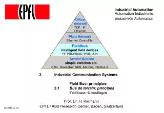
2.1.1 Market • 2.1 Instrumentation • 2.1.1 Market • 2.1.2 Binary instruments • 2.1.3 Analog Instruments • 2.1.4 Actuators • 2.1.5 Transducers • 2.1.6 Instrumentation diagrams • 2.1.7 Protection classes • 2.2 Control • 2.3 Programmable Logic Controllers
The instrumentation market Global Process Automation and Process Instrumentation Market, 2013-2018 ($Billion) Source: Markets And Markets - Process Automation Market & Instrumentation Market – By Technology (SCADA, PLC, DCS, MES), Communication (Profibus, Fieldbus, Wireless HART, ISA100), Transmitter (Flow, Temperature, Level, Pressure) - Analysis and Forecast (2013 – 2018)
Example Nuclear power plant Nombre de capteurs et d’actionneurs pour une tranche et selon les paliers (number of sensors and actors for each slice and according to the level) Jean CHABERT, Bernard APPELL, Guy GUESNIER, 1998
Concepts • instruments = sensors (capteurs, Messgeber) andactuators (actionneurs, Stellglieder) • binary (on/off) and analog (continuous) instruments are distinguished. • industrial conditions: • temperature range commercial: (0°C to +70°C) industry (-40°C..+85°C)extended industrial(–40°C..+125°C) • mechanical resilience (shocks and vibrations) EN 60068 • protection: Electro-Magnetic (EM)-disturbances EN 55022, EN55024) • protection: water and moisture (IP67=completely sealed, IP20 = normal) • protection: NEMP (Nuclear EM Pulse) - water distribution, civil protection • mounting and replacement • robust connectors • power: DC mostly 24V= because of battery back-up, sometimes 48V=
2.1.2 Binary Instruments • 2.1 Instrumentation • 2.1.1 Market • 2.1.2 Binary instruments • 2.1.3 Analog Instruments • 2.1.4 Actors • 2.1.5 Transducers • 2.1.6 Instrumentation diagrams • 2.1.7 Protection classes • 2.2 Control • 2.3 Programmable Logic Controllers
Binary position measurement • binary sensors (Geber, "Initiator", indicateur "tout ou rien"): • micro-switch (Endschalter, contact fin de course) +cheap, -wear, bouncing • optical sensor (Lichtschranke, barrière optique) +reliable, -dust or liquid sensitive • magnetic sensor (Näherungsschalter, détecteur de proximité) +dust-insensitive, - magnetic
Binary Signal processing • Physical attachment • Level adaptation, • Galvanical separation • EMC barrier (against sparks, radio, disturbances) • Acquisition • Convert to standard levels • Relay contacts 24V (most frequent), 48V, 110V (electrical substations) • Electronic signals 24V —>10V-60V, • Output: 0..24V@100mA • Counter inputs: Gray, BCD or binary • Processing • Filtering (e.g. 0..8 ms filter), • Plausibility (Antivalenz, Antivalence), • Bounce-free (Entprellen, Anti-rebond)
2.1.3 Analog Instruments • 2.1 Instrumentation • 2.1.1 Market • 2.1.2 Binary instruments • 2.1.3 Analog Instruments • 2.1.3.1 Position and speed • 2.1.3.2 Temperature • 2.1.3.3 Hydraulic • 2.1.4 Actors • 2.1.5 Transducers • 2.1.6 Instrumentation diagrams • 2.1.7 Protection classes • 2.2 Control • 2.3 Programmable Logic Controllers
Precision (repeatability) and accuracy (deviation) Not precise Accurate Not precise Not accurate Precise Accurate Precise Not accurate Accuracy is a consequence of systematic errors (or bad calibration) accuracy and precision may depends on time (drift)
Resolution • Resolution expresses how many different levels can be distinguished • resolution is the smallest number that can be displayed or recorded by the measurement device. • Example • A reading device that has a specified accuracy of ±0.015% will actually give a reading that is between 0.99985 and 1.00015 times the actual value. • measuring 1 volt within ±0.015% accuracy requires a 6-digit instrument capable of displaying five decimal places. The fifth decimal place represents 10 microvolts, giving this instrument a resolution of 10 microvolts.
Precision, Accuracy and Precision Summary • PRECISON • How reproducible or close identical measurements will be reported as a percentage of full scale. • ACCURACY • The ability of the instrument to measure a quantity to the absolute true and correct value. • RESOLUTION • The smallest unit of measure or the smallest change that can be displayed or recorded by an instrument (sometimes referred to as granularity)
2.1.3.1 Analog mechanical position +cheap, -wear, bad resolution potentiometer capacitive balanced transformer (LVDT) (linear or sin/cos encoder) strain gauges piezo-electric +cheap, -bad resolution +reliable, robust - small displacements +reliable, very small displacements +extremely small displacements
Variable differential transformer (LVDT) – Linear displacement The LVDT is a variable-reluctance device, where a primary centercoil establishes a magnetic flux that is coupled through a mobilearmature to a symmetrically-wound secondary coil on either sideof the primary. Two components comprise the LVDT: the mobile armature andthe outer transformer windings. The secondary coils areseries-opposed; wound in series but in opposite directions. When the moving armature is centered between the two series-opposed secondaries, equal magnetic flux couples into both secondaries; the voltage induced in one half of the secondary winding is 180 degrees out-of-phase with the voltage induced in the other half of the secondary winding. When the armature is moved out of that position, a voltage proportional to the displacement appears source: www.sensorland.com
Capacitive angle or position measurement A C = ε ≈ a d movable capacitance is evaluated by modifying the frequency of an oscillator a fixed
Small position measurement: strain gauges Dehnungsmessstreifen (DMS),jauges de contrainte Principle: the resistance of a wire with resistivity ρ increases when this wire is stretched: A ρ = resistivity l l' l2 R = r ≈ l2 = r A V l" volume = constant, r = constant measurement using a Wheatstone bridge (if U0 = 0: R1R4 = R2R3) R1 measure R3 U temperature compensation by “dummy” gauges Uo R2 compensation R4 frequently used in buildings, bridges, dams for detecting movements.
Piezo-electrical effect Piezoelectric materials (crystals) change form when an electrical field is applied to them. Conversely, piezoelectric materials produce an electrical field when deformed. • Quartz transducers exhibit remarkable properties that justify their large scale use in research, development, production and testing. They are extremely stable, rugged and compact. • Of the large number of piezoelectric materials available today, quartz is employed preferentially in transducer designs because of the following excellent properties: • high material stress limit, around 100 MPa (~ 14 km water depth) • temperature resistance (up to 500C) • very high rigidity, high linearity and negligible hysteresis • almost constant sensitivity over a wide temperature range • ultra high insulation resistance (10+14 ohms) allowing low frequency measurements (<1 Hz) source: Kistler
Principle of optical angle encoder Optical encoders operate by means of a grating that moves between a light source and a detector. The detector registers when light passes through the transparent areas of the grating. For increased resolution, the light source is collimated and a mask is placed between the grating and the detector. The grating and the mask produce a shuttering effect, so that only when their transparent sections are in alignment is light allowed to pass to the detector (Moiré pattern). An incremental encoder generates a pulse for a given increment of shaft rotation (rotary encoder), or a pulse for a given linear distance travelled (linear encoder). Total distance travelled or shaft angular rotation is determined by counting the encoder output pulses. An absolute encoder has a number of output channels, such that every shaft position may be described by its own unique code. The higher the resolution the more output channels are required. courtesy Parker Motion & Control
Incremental angle encoder Photo: Lenord & Bauer open mounted Photo: Baumer
Absolute digital position: Gray encoder binary code: if all bits were to change at about the same time: glitches 0 1 2 3 4 5 6 7 8 9 10 11 12 13 14 15 LSB MSB Gray code: only one bit changes at a time: no glitch 0 1 2 3 4 5 6 7 8 9 10 11 12 13 14 15 LSB courtesy Parker Motion & Control MSB Gray disk (8 bit)