Download
1 / 71
900 likes | 1.51k Views
ECONOMICS 5e. Michael Parkin. CHAPTER 12 Perfect Competition. Learning Objectives. Define perfect competition Explain how price and output are determined in a competitive industry Explain why firms sometimes shut down temporarily and lay off workers. Learning Objectives (cont.).

E N D
ECONOMICS 5e Michael Parkin CHAPTER 12Perfect Competition
Learning Objectives • Define perfect competition • Explain how price and output are determined in a competitive industry • Explain why firms sometimes shut down temporarily and lay off workers
Learning Objectives (cont.) • Explain why firms enter and leave an industry • Predict the effects of a change in demand and of a technological advance • Explain why perfect competition is efficient
Learning Objectives • Define perfect competition • Explain how price and output are determined in a competitive industry • Explain why firms sometimes shut down temporarily and lay off workers
Perfect Competition Characteristics of Perfect Competition • Many firms, each selling an identical product. • Many buyers. • No restrictions on entry into the industry.
Perfect Competition Characteristics of Perfect Competition • Firms in the industry have no advantage over potential new entrants. • Firms and buyers are well informed about prices of the products of each firm in the industry.
Perfect Competition As a result of these characteristics, perfect competitors are price takers. Price takers Firms that cannot influence the price of a good or service.
Learning Objectives • Define perfect competition • Explain how price and output are determined in a competitive industry • Explain why firms sometimes shut downtemporarily and lay off workers
Economic Profit and Revenue Thefirm’s goal is to maximize economic profit. Total cost is the opportunity cost - including normal profit.
Economic Profit and Revenue Total revenue is the value of a firm’s sales. • Total revenue = P Q Marginal revenue(MR) • Change in total revenue resulting from a one-unit increase in quantity sold. Average revenue(AR) • Total revenue divided by the quantity sold—revenue per unit sold. In perfect competition, Price = MR = AR
Economic Profit and Revenue Suppose Sidney sells his sweaters in a perfectly competitive market.
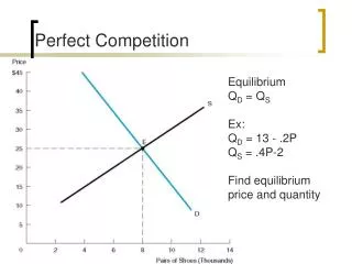
Demand, Price, and Revenuein Perfect Competition Quantity Price Marginal Average sold (P) Total revenue revenue (Q) (dollars revenue (AR = TR/Q (sweaters per TR = P Q (dollars per (dollars per day) sweater) (dollars) additional sweater) per sweater) 8 25 9 25 10 25
Demand, Price, and Revenuein Perfect Competition Quantity Price Marginal Average sold (P) Total revenue revenue (Q) (dollars revenue (AR = TR/Q (sweaters per TR = P Q (dollars per (dollars per day) sweater) (dollars) additional sweater) per sweater) 8 25 200 9 25 225 10 25 250
Demand, Price, and Revenuein Perfect Competition Quantity Price Marginal Average sold (P) Total revenue revenue (Q) (dollars revenue (AR = TR/Q (sweaters per TR = P Q (dollars per (dollars per day) sweater) (dollars) additional sweater) per sweater) 8 25 200 9 25 225 10 25 250 25 25
Demand, Price, and Revenuein Perfect Competition Quantity Price Marginal Average sold (P) Total revenue revenue (Q) (dollars revenue (AR = TR/Q (sweaters per TR = P Q (dollars per (dollars per day) sweater) (dollars) additional sweater) per sweater) 8 25 200 25 9 25 225 25 10 25 250 25 25 25
Sidney’s demand curve TR MR S a D Demand, Price, and Revenuein Perfect Competition Sidney’s demand and marginal revenue Sweater market Sidney’s total revenue 50 50 Price (dollars per sweater) Price (dollars per sweater) Total revenue (dollar per day) Market demand curve 25 225 25 0 9 20 0 10 20 0 9 20 Quantity (thousands of sweaters per day) Quantity (sweaters per day) Quantity (sweaters per day)
Learning Objectives • Define perfect competition • Explain how price and output are determined in a competitive industry • Explain why firms sometimes shut down temporarily and lay off workers
The Firm’s Decisions inPerfect Competition A firm’s task is to make the maximum economic profit possible, given the constraints it faces. In order to do so, the firm must make two decisions in the short-run, and two in the long-run.
The Firm’s Decisions inPerfect Competition Short-run A time frame in which each firm has a given plant and the number of firms in the industry is fixed Long-run A time frame in which each firm can change the size of its plant and decide to enter the industry.
The Firm’s Decisions inPerfect Competition In the short-run, the firm must decide: • Whether to produce or to shut down. • If the decision is to produce, what quantity to produce.
The Firm’s Decisions inPerfect Competition In the long-run, the firm must decide: • Whether to increase of decrease its plant size. • Whether to stay in the industry or leave it. We will first address the short-run.
Total Revenue, Total Cost, and Economic Profit Quantity Total Total Economic (Q) revenue cost profit (sweaters (TR) (TC) (TR – TC) Per day) (dollars) (dollars) (dollars) 0 0 1 25 2 50 3 75 4 100 5 125 6 150 7 175 8 200 9 225 10 250 11 275 12 300 13 325
Total Revenue, Total Cost,and Economic Profit Quantity Total Total Economic (Q) revenue cost profit (sweaters (TR) (TC) (TR – TC) Per day) (dollars) (dollars) (dollars) 0 0 22 1 25 45 2 50 66 3 75 85 4 100 100 5 125 114 6 150 126 7 175 141 8 200 160 9 225 183 10 250 210 11 275 245 12 300 300 13 325 360
Total Revenue, Total Cost,and Economic Profit Quantity Total Total Economic (Q) revenue cost profit (sweaters (TR) (TC) (TR – TC) Per day) (dollars) (dollars) (dollars) 0 0 22 -22 1 25 45 -20 2 50 66 -16 3 75 85 -10 4 100 100 0 5 125 114 11 6 150 126 24 7 175 141 24 8 200 160 40 9 225 183 42 10 250 210 40 11 275 245 30 12 300 300 0 13 325 360 -35
TC Economic loss Economic profit = TR - TC Economic loss Total Revenue, Total Cost,and Economic Profit TR 300 Total revenue & total cost (dollars per day) 225 183 100 0 4 9 12 Quantity (sweaters per day)
Economic profit Economic loss Profit maximizing quantity Total Revenue, Total Cost,and Economic Profit Economic profit/loss 42 Profit/loss (dollars per day) 20 0 Quantity (sweaters per day) 4 9 12 -20 Profit/ loss -40
Marginal Analysis Using marginal analysis, a comparison is made between a units marginal revenue and marginal cost.
Marginal Analysis If MR > MC, the extra revenue from selling one more unit exceeds the extra cost. • The firm should increase output to increase profit. If MR < MC, the extra revenue from selling one more unit is less than the extra cost. • The firm should decrease output to increase profit. If MR = MC economic profit is maximized.
Profit-Maximizing Output Marginal Marginal revenue cost Quantity Total (MR) Total (MC) Economic (Q) revenue (dollars per cost (dollars per profit (sweaters (TR) additional (TC) additional (TR – TC) per day) (dollars) sweater) (dollars sweater) (dollars) 7 175 8 200 9 225 10 250 11 275
Profit-Maximizing Output Marginal Marginal revenue cost Quantity Total (MR) Total (MC) Economic (Q) revenue (dollars per cost (dollars per profit (sweaters (TR) additional (TC) additional (TR – TC) per day) (dollars) sweater) (dollars sweater) (dollars) 7 175 8 200 9 225 10 250 11 275 25 25 25 25
Profit-Maximizing Output Marginal Marginal revenue cost Quantity Total (MR) Total (MC) Economic (Q) revenue (dollars per cost (dollars per profit (sweaters (TR) additional (TC) additional (TR – TC) per day) (dollars) sweater) (dollars sweater) (dollars) 7 175 141 8 200 160 9 225 183 10 250 210 11 275 245 25 25 25 25
Profit-Maximizing Output Marginal Marginal revenue cost Quantity Total (MR) Total (MC) Economic (Q) revenue (dollars per cost (dollars per profit (sweaters (TR) additional (TC) additional (TR – TC) per day) (dollars) sweater) (dollars sweater) (dollars) 7 175 141 8 200 160 9 225 183 10 250 210 11 275 245 25 25 25 25 19 23 27 35
Profit-Maximizing Output Marginal Marginal revenue cost Quantity Total (MR) Total (MC) Economic (Q) revenue (dollars per cost (dollars per profit (sweaters (TR) additional (TC) additional (TR – TC) per day) (dollars) sweater) (dollars sweater) (dollars) 7 175 141 34 8 200 160 40 9225183 42 10 250 210 40 11 275 245 30 25 25 25 25 19 23 27 35
Profit- maximization point MC Loss from 10th sweater MR Profit from 9th sweater Profit-Maximizing Output 30 25 Marginal revenue & marginal cost (dollars per day) 20 10 0 8 9 10 Quantity (sweaters per day)
The Firm’s Short-Run Supply Curve Fixed costs must be paid in the short-run. Variable-costs can be avoided by laying off workers and shutting down. Firms shut down if price falls below the minimum of average variable cost.
MC = S MR2 MR1 Shutdown point AVC s MR0 A Firm’s Supply Curve 31 Marginal revenue & marginal cost (dollars per day) 25 17 0 7 9 10 Quantity (sweaters per day)
S s A Firm’s Supply Curve 31 Marginal revenue & marginal cost (dollars per day) 25 17 0 7 9 10 Quantity (sweaters per day)
Short-Run Industry Supply Curve Short-run industry supply curve Shows the quantity supplied by the industry at each price when the plant size of each firm and the number of firms remain constant. It is constructed by summing the quantities supplied by the individual firms.
Industry Supply Curve Quantity supplied Quantity supplied Price by Sidney by industry (dollars (sweaters (sweaters per sweater) per day) per day) a 17 0 or 7 0 to 7,000 b 2 8 8,000 c 25 9 9,000 d 31 10 10,000
S1 Industry Supply Curve 40 Price (dollars per sweater) 30 20 0 6 7 8 9 10 Quantity (thousands of sweaters per day)
Output, Price, and Profitin Perfect Competition Industry demand and industry supply determine the market price and industry output. Changes in demand bring changes to short-run industry equilibrium.
D2 D3 Short-Run Equilibrium Increase in demand: price rises and firms increase production S Price (dollars per sweater) 25 Decrease in demand: price falls and firms decrease production 20 17 D1 0 6 7 8 9 10 Quantity (thousands of sweaters per day)
Profits and Losses in the Short-Run At short-run equilibrium firms may: • Earn a profit • Break even • Incur an economic loss.
Profits and Losses in the Short-Run If price equals average total cost a firm breaks even. If price exceeds average total cost, a firm makes an economic profit. If price is less than average total cost, a firm incurs an economic loss.
Break-even point AR = MR Three Possible Profit Outcomesin the Short-Run Normal profit 30.00 MC ATC Price (dollars per chip) 25.00 20.00 15.00 0 8 10 Quantity (millions of chips per year)
AR = MR Economic Profit Three Possible Profit Outcomesin the Short-Run Economic profit 30.00 MC ATC Price (dollars per chip) 25.00 20.33 15.00 0 9 10 Quantity (millions of chips per year)
Economic loss AR = MR Three Possible Profit Outcomesin the Short-Run Economic loss 30.00 MC ATC Price (dollars per chip) 25.00 20.14 17.00 0 7 10 Quantity (millions of chips per year)
Learning Objectives (cont.) • Explain why firms enter and leave an industry • Predict the effects of a change in demand and of a technological advance • Explain why perfect competition is efficient
Long-Run Adjustments Forces in a competitive industry ensure only one of these situations is possible in the long-run. Competitive industries adjust in two ways: • Entry and exit • Changes in plant size
Entry and Exit The prospect of persistent profit or loss causes firms to enter or exit an industry. If firms are making economic profits, other firms enter the industry. If firms are making economic losses, some of the existing firms exit the industry.