Download
1 / 36
360 likes | 364 Views
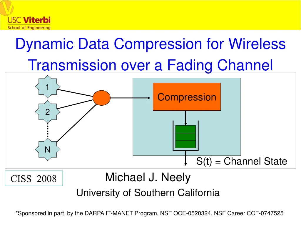
1. Compression. 2. N. S(t) = Channel State. Dynamic Data Compression for Wireless Transmission over a Fading Channel. Michael J. Neely University of Southern California. CISS 2008. *Sponsored in part by the DARPA IT-MANET Program, NSF OCE-0520324, NSF Career CCF-0747525. 1.

E N D
1 Compression 2 N S(t) = Channel State Dynamic Data Compression for WirelessTransmission over a Fading Channel Michael J. Neely University of Southern California CISS 2008 *Sponsored in part by the DARPA IT-MANET Program, NSF OCE-0520324, NSF Career CCF-0747525
1 Compression 2 N S(t) = Channel State -Random Packet Arrivals A(t) -Stochastic Channel S(t) -Data must be Compressed, Stored, and Transmitted Both Compression and Transmission expend power! Goal: Minimize Total Average Power Expenditure Ptot = Pcomp + Ptran (signal processing consumes power)
Compression Operation: 1 Y(A(t), K(t)) 2 N Timeslotted System: t = {0,1, 2, 3,…} A(t) = # packet arrivals at time t (fixed packets size B bits, A(t) {0, 1, …, N} ) K(t) = Compression Decision Option at time t (K(t) {0, 1, …, K}) Y(A(t), K(t)) = Compression Function = Random bit size output after compression
Compression Operation: 1 Y(A(t), K(t)) 2 N Timeslotted System: t = {0,1, 2, 3,…} A(t) = # packet arrivals at time t (fixed packets size B bits, A(t) {0, 1, …, N} ) K(t) = Compression Decision Option at time t (K(t) {0, 1, …, K}) Y(A(t), K(t)) = Compression Function Example: A(t) = 2, K(t)=k Y(A(t), K(t)) = ?? (random output) Pcomp(t) = ?? (random output)
Compression Operation: 1 Y(A(t), K(t)) 2 N Timeslotted System: t = {0,1, 2, 3,…} A(t) = # packet arrivals at time t (fixed packets size B bits, A(t) {0, 1, …, N} ) K(t) = Compression Decision Option at time t (K(t) {0, 1, …, K}) Y(A(t), K(t)) = Compression Function Example: A(t) = 2, K(t)=k Y(A(t), K(t)) = ?? (random output) Pcomp(t) = ?? (random output)
Compression Operation: 1 Y(A(t), K(t)) 2 N Timeslotted System: t = {0,1, 2, 3,…} A(t) = # packet arrivals at time t (fixed packets size B bits, A(t) {0, 1, …, N} ) K(t) = Compression Decision Option at time t (K(t) {0, 1, …, K}) Y(A(t), K(t)) = Compression Function Example: A(t) = 2, K(t)=k Y(A(t), K(t)) = ?? (random output) Pcomp(t) = ?? (random output)
Compression Operation: 1 Y(A(t), K(t)) 2 N Timeslotted System: t = {0,1, 2, 3,…} A(t) = # packet arrivals at time t (fixed packets size B bits, A(t) {0, 1, …, N} ) K(t) = Compression Decision Option at time t (K(t) {0, 1, …, K}) Y(A(t), K(t)) = Compression Function Example: A(t) = 2, K(t)=k Y(A(t), K(t)) = ?? (random output) Pcomp(t) = ?? (random output)
Compression Operation: 1 Y(A(t), K(t)) 2 1.1 N Timeslotted System: t = {0,1, 2, 3,…} A(t) = # packet arrivals at time t (fixed packets size B bits, A(t) {0, 1, …, N} ) K(t) = Compression Decision Option at time t (K(t) {0, 1, …, K}) Y(A(t), K(t)) = Compression Function Example: A(t) = 2, K(t)=k Y(A(t), K(t)) = (1.1)B bits (random output) Pcomp(t) = .2 mW (random output)
Compression Operation: 1 Y(A(t), K(t)) 2 N Timeslotted System: t = {0,1, 2, 3,…} A(t) = # packet arrivals at time t (fixed packets size B bits, A(t) {0, 1, …, N} ) K(t) = Compression Decision Option at time t (K(t) {0, 1, …, K}) Y(A(t), K(t)) = Compression Function Example 2: A(t) = 2, K(t)=k Y(A(t), K(t)) = ?? (random output) Pcomp(t) = ?? (random output)
Compression Operation: 1 Y(A(t), K(t)) 2 N Timeslotted System: t = {0,1, 2, 3,…} A(t) = # packet arrivals at time t (fixed packets size B bits, A(t) {0, 1, …, N} ) K(t) = Compression Decision Option at time t (K(t) {0, 1, …, K}) Y(A(t), K(t)) = Compression Function Example 2: A(t) = 2, K(t)=k Y(A(t), K(t)) = ?? (random output) Pcomp(t) = ?? (random output)
Compression Operation: 1 Y(A(t), K(t)) 2 N Timeslotted System: t = {0,1, 2, 3,…} A(t) = # packet arrivals at time t (fixed packets size B bits, A(t) {0, 1, …, N} ) K(t) = Compression Decision Option at time t (K(t) {0, 1, …, K}) Y(A(t), K(t)) = Compression Function Example 2: A(t) = 2, K(t)=k Y(A(t), K(t)) = ?? (random output) Pcomp(t) = ?? (random output)
Compression Operation: 1 Y(A(t), K(t)) 2 N Timeslotted System: t = {0,1, 2, 3,…} A(t) = # packet arrivals at time t (fixed packets size B bits, A(t) {0, 1, …, N} ) K(t) = Compression Decision Option at time t (K(t) {0, 1, …, K}) Y(A(t), K(t)) = Compression Function Example 2: A(t) = 2, K(t)=k Y(A(t), K(t)) = ?? (random output) Pcomp(t) = ?? (random output)
Compression Operation: 1 Y(A(t), K(t)) 2 0.9 N Timeslotted System: t = {0,1, 2, 3,…} A(t) = # packet arrivals at time t (fixed packets size B bits, A(t) {0, 1, …, N} ) K(t) = Compression Decision Option at time t (K(t) {0, 1, …, K}) Y(A(t), K(t)) = Compression Function Example 2: A(t) = 2, K(t)=k Y(A(t), K(t)) = (0.9)B bits (random output) Pcomp(t) = .3 mW (random output)
Compression Operation: 1 Y(A(t), K(t)) 2 N Timeslotted System: t = {0,1, 2, 3,…} A(t) = # packet arrivals at time t (fixed packets size B bits, A(t) {0, 1, …, N} ) K(t) = Compression Decision Option at time t (K(t) {0, 1, …, K}) Y(A(t), K(t)) = Compression Function Example 3: A(t) = 3, K(t)=k Y(A(t), K(t)) = ?? (random output) Pcomp(t) = ?? (random output)
Compression Operation: 1 Y(A(t), K(t)) 2 N Timeslotted System: t = {0,1, 2, 3,…} A(t) = # packet arrivals at time t (fixed packets size B bits, A(t) {0, 1, …, N} ) K(t) = Compression Decision Option at time t (K(t) {0, 1, …, K}) Y(A(t), K(t)) = Compression Function Example 3: A(t) = 3, K(t)=k Y(A(t), K(t)) = ?? (random output) Pcomp(t) = ?? (random output)
Compression Operation: 1 Y(A(t), K(t)) 2 N Timeslotted System: t = {0,1, 2, 3,…} A(t) = # packet arrivals at time t (fixed packets size B bits, A(t) {0, 1, …, N} ) K(t) = Compression Decision Option at time t (K(t) {0, 1, …, K}) Y(A(t), K(t)) = Compression Function Example 3: A(t) = 3, K(t)=k Y(A(t), K(t)) = ?? (random output) Pcomp(t) = ?? (random output)
Compression Operation: 1 Y(A(t), K(t)) 2 N Timeslotted System: t = {0,1, 2, 3,…} A(t) = # packet arrivals at time t (fixed packets size B bits, A(t) {0, 1, …, N} ) K(t) = Compression Decision Option at time t (K(t) {0, 1, …, K}) Y(A(t), K(t)) = Compression Function Example 3: A(t) = 3, K(t)=k Y(A(t), K(t)) = ?? (random output) Pcomp(t) = ?? (random output)
Compression Operation: 1 Y(A(t), K(t)) 2 1.6 N Timeslotted System: t = {0,1, 2, 3,…} A(t) = # packet arrivals at time t (fixed packets size B bits, A(t) {0, 1, …, N} ) K(t) = Compression Decision Option at time t (K(t) {0, 1, …, K}) Y(A(t), K(t)) = Compression Function Example 3: A(t) = 3, K(t)=k Y(A(t), K(t)) = (1.6)B bits (random output) Pcomp(t) = .4 mW (random output)
Good rate m Med Bad power P Transmission Operation: 1 Y(A(t), K(t)) 2 N S(t) = Channel State S(t) = Current Channel State on slot t Example: S(t) {“Good”, “Med”, “Bad”} S(t) {attenuation, 0 < S(t) < 1} Ptran(t) = Power Decision on slot t (P = set of power options) Example:P {0 < p < Pmax} or P {0, Pmax/2, Pmax} m(t) = C(Ptran(t), S(t)) = transmission rate on slot t rate-power curve
Good rate m Med Bad power P Transmission Operation: 1 Y(A(t), K(t)) 2 N S(t) = Channel State S(t) = Current Channel State on slot t Example: S(t) {“Good”, “Med”, “Bad”} S(t) {attenuation, 0 < S(t) < 1} Ptran(t) = Power Decision on slot t (P = set of power options) Example:P {0 < p < Pmax} or P {0, Pmax/2, Pmax} m(t) = C(Ptran(t), S(t)) = transmission rate on slot t rate-power curve
Ptot = Pcomp + Ptran 1 Y(A(t), K(t)) 2 Q(t) ~ bits N Queueing Dynamics: Q(t+1) = max[Q(t) - m(t), 0] + R(t) m(t) = C(Ptran(t), S(t)) , R(t) = Y(A(t), K(t)) Goal: Design a joint strategy for choosing compression and transmission decisions K(t), Ptran(t) over time to support all traffic and minimize total average power. [Also want low delay!]
Intuition:Consider a trivial case where all of the following hold… Static Channel: S(t) = Constant Linear rate-power curve: C(P) = aP Raw Data Rate small: E{A(t)}B < mmax= aPmax If all 3 hold, easy to show Ptran proportional to bits transmitted, and decision is trivial: choose K(t) = k {0,…,K} that minimizes: f(a, k) + m(a,k)/a If one or more of the above fail, decision is non-trivial!
Prior Experimental Work in this case: Barr, Asanovic “Energy Aware Lossless Data compression” [2003] 2. Sadler, Martonosi “Data Compression algorithms for energy-constrained devices” [SenSys2006] Data Compression an important problem! [Richard Baraniuk’s Plenary talk was totally cool!] Intelligent Compression Can Significantly Improve Power Expenditure.
Defining Optimality: The h*(r) and g*(r) functions Assume: - # arrivals A(t) iid over slots, pA(a) = Pr[A(t) = a] - S(t) iid over slots, ps = Pr[S(t) = s] Distributions pA(a) and ps are potentially unknown to controller Min bit rate out of compressor Max time avg. transmission rate (assume rmin < rmax)
Defining Optimality: The h*(r) and g*(r) functions Assume: - # arrivals A(t) iid over slots, pA(a) = Pr[A(t) = a] - S(t) iid over slots, ps = Pr[S(t) = s] Distributions pA(a) and ps are potentially unknown to controller Intuitively: There are two reasons to compress data: To stabilize queue, we may need to compress (if raw input rate > rmax ) ii) Power spent compressing can reduce trans. power.
Defining Optimality: The h*(r) and g*(r) functions h*(r) = minimum Pcomp to yield compressor output rate r. g*(r) = minimum Ptran to yield avg. transmission rate r. Min h such that: Min g such that: (optimizing over all stationary randomized opportunistic policies) h*(r) g*(r) rate r rmax rate r rmin
Theorem (characterizing minimum avg. power): Any stabilizing policy yields avg. power such that: Pcomp + Ptran P* > av Where P* is the min avg. power and satisfies: av Minimize: h*(r) + g*(r) Subject to: rmin < r < min[rmax, BE{A(t)}] Total avg power rate r rmin min[rmax, BE{A(t)}]
Want a dynamic control algorithm to minimize power… Use Joint Lyapunov Stability + Performance Optimization Technique for Stochastic Network Optimization: -Georgiadis, Neely, Tassiulas [NOW F&T in Networking, 2006] -Neely [Phd thesis 2003, Infocom 2005, IT 2006] -See also related technique in Stolyar [Queueing Systems 2005] Lyapunov Function: L(Q) = (1/2) Q2 Lyapunov Drift:D(Q(t)) = E{L(Q(t+1)) - L(Q(t)) | Q(t)} Technique: Every slot, observe Q(t), take control action to minimize (for a given constant V>0): D(Q(t)) + VE{Cost(t)| Q(t)} Theorem: 1) E{Q} < O(V) 2) E{Cost(actual) - Cost(optimal)} < O(1/V)
1 Y(A(t), K(t)) 2 N S(t) = Channel State The Dynamic Compression and Transmission Algorithm: Compression: On slot t, observe A(t). Choose K(t) such that: Transmission: On slot t, observe S(t). Choose Ptran(t) such that: Q Q
1 Y(A(t), K(t)) 2 N S(t) = Channel State Q Concluding Theorem (Performance): For any V>0 we have: B = (1/2)[mmax2 + B2E{A2}]
1 Y(A(t), K(t)) 2 N S(t) = Channel State Q P* av Concluding Theorem (Performance): For any V>0 we have: Avg Power Avg Delay V V
1 Y(A(t), K(t)) 2 N S(t) = Channel State Q P* av Concluding Theorem (Performance): For any V>0 we have: Avg Power Avg Delay V V
1 Y(A(t), K(t)) 2 N S(t) = Channel State Q P* av Concluding Theorem (Performance): For any V>0 we have: Avg Power Avg Delay V V
1 Y(A(t), K(t)) 2 N S(t) = Channel State Q P* av Concluding Theorem (Performance): For any V>0 we have: Avg Power Avg Delay V V
1 Y(A(t), K(t)) 2 N S(t) = Channel State Q P* av Concluding Theorem (Performance): For any V>0 we have: Avg Power Avg Delay V V
1 Y(A(t), K(t)) 2 N S(t) = Channel State Q P* av Concluding Theorem (Performance): For any V>0 we have: Avg Power Avg Delay V V