Computational Genomics Lecture #3

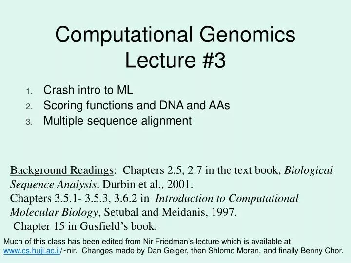
1. Computational GenomicsLecture #3 Crash intro to ML Scoring functions and DNA and AAs Multiple sequence alignment Background Readings: Chapters 2.5, 2.7 in the text book, Biological Sequence Analysis, Durbin et al., 2001. Chapters 3.5.1- 3.5.3, 3.6.2 in Introduction to Computational Molecular Biology, Setubal and Meidanis, 1997. Chapter 15 in Gusfield’s book. Much of this class has been edited from Nir Friedman’s lecture which is available at www.cs.huji.ac.il/~nir. Changes made by Dan Geiger, then Shlomo Moran, and finally Benny Chor.

2. Scoring Functions, Reminder • So far, we discussed dynamic programming algorithms for • global alignment • local alignment • All of these assumed a scoring function: that determines the value of perfect matches, substitutions, insertions, and deletions.

3. Where does the scoring function come from ? We have defined an additive scoring function by specifying a function ( ,  ) such that • (x,y) is the score of replacingx by y • (x,-) is the score of deletingx • (-,x) is the score of insertingx But how do we come up with the “correct” score ? Answer: By encoding experience of what are similar sequences for the task at hand. Similarity depends on time, evolution trends, and sequence types.

4. Why probability setting is appropriate to define and interpret a scoring function ? • Similarity is probabilistic in nature because biological changes like mutation, recombination, and selection, are random events. • We could answer questions such as: • How probable it is for two sequences to be similar? • Is the similarity found significant or spurious? • How to change a similarity score when, say, mutation rate of a specific area on the chromosome becomes known ?

5. A Probabilistic Model • For starters, will focus on alignment without indels. • For now, we assume each position (nucleotide /amino-acid) is independent of other positions. • We consider two options: M: the sequences are Matched(related) R: the sequences are Random (unrelated)

6. Unrelated Sequences • Our random model R of unrelated sequences is simple • Each position is sampled independently from a distribution over the alphabet  • We assume there is a distribution q() that describes the probability of letters in such positions. • Then:

7. Related Sequences • We assume that each pair of aligned positions (s[i],t[i]) evolved from a common ancestor • Let p(a,b) be a distribution over pairs of letters. • p(a,b) is the probability that some ancestral letterevolved into this particular pair of letters. Compare to:

8. Odd-Ratio Test for Alignment If Q > 1, then the two strings s and t are more likely to be related (M) than unrelated (R). If Q < 1, then the two strings s and t are more likely to be unrelated (R) than related (M).

9. Log Odd-Ratio Test for Alignment Taking logarithm of Q yields Score(s[i],t[i]) If log Q > 0, then s and t are more likely to be related. If log Q < 0, then they are more likely to be unrelated. How can we relate this quantity to a score function ?

10. Probabilistic Interpretation of Scores • We define the scoring function via • Then, the score of an alignment is the log-ratio between the two models: • Score > 0 Model is more likely • Score < 0 Random is more likely

11. Modeling Assumptions • It is important to note that this interpretation depends on our modeling assumption!! • For example, if we assume that the letter in each position depends on the letter in the preceding position, then the likelihood ratio will have a different form. • If we assume, for proteins, some joint distribution of letters that are nearby in 3D space after protein folding, then likelihood ratio will again be different.

12. Estimating Probabilities • Suppose we are given a long string s[1..n] of letters from  • We want to estimate the distribution q(·) that generated the sequence • How should we go about this? We build on the theory of parameter estimation in statistics using either maximum likelihood (today) estimation or the Bayesian approach (later on).

13. Estimating q() • Suppose we are given a long string s[1..n] of letters from  • scan be the concatenation of all sequences in our database • We want to estimate the distribution q() • That is, q is defined per single letters Likelihood function:

14. Estimating q()(cont.) How do we define q? Intuitively Likelihood function: ML parameters (Maximum Likelihood)

15. Crash Course on Maximum Likelihood: Binomial Experiment When tossed, this device (“thumbtack”) can land in one of two positions: Head or Tail Head Tail • We denote by  the (unknown) probability P(H). Estimation task: • Given a sequence of toss samples x[1], x[2], …, x[M] we want to estimate the probabilities P(H)=  and P(T) = 1 - 

16. i.i.d. samples Statistical Parameter Fitting • Consider instances x[1], x[2], …, x[M] , such that • The set of values that x can take is known • Each is sampled from the same distribution • Each sampled independently of the rest • The task is to find a vector of parameters  that have generated the given data. This vector parameter  can be used to predict future data.

17. L()  0 0.2 0.4 0.6 0.8 1 The Likelihood Function • How good is a particular ?It depends on how likely it is to generate the observed data The likelihood for the sequence H,T,T,H,H is

18. Sufficient Statistics • To compute the likelihood in the thumbtack example we only require NH and NT (the number of heads and the number of tails) • NH and NTare sufficient statistics for the binomial distribution

19. Formally, s(D) is a sufficient statistics if for any two datasets DandD’ • s(D) = s(D’ )LD() = LD’ () Datasets Statistics Sufficient Statistics • A sufficient statistic is a function of the data that summarizes the relevant information for the likelihood

20. Maximum Likelihood Estimation MLE Principle: Choose parameters that maximize the likelihood function • This is one of the most commonly used estimators in statistics • Intuitively appealing • One usually maximizes the log-likelihood function defined as lD() = loge LD()

21. L() 0 0.2 0.4 0.6 0.8 1 (Which coincides with what one would expect) Example: (NH,NT ) = (3,2) MLE estimate is 3/5 = 0.6 Example: MLE in Binomial Data • Applying the MLE principle (taking derivative) we get

22. Estimating p(·,·) Intuition: • Find pair of aligned sequences s[1..n], t[1..n], • Estimate probability of pairs: • The sequences s and t can be the concatenation of many aligned pairs from the database Number of times a is aligned with b in (s,t)

23. Problems in Estimating p(·,·) • How do we find pairs of aligned sequences? • How far is the ancestor ? • earlier divergence  low sequence similarity • recent divergence  high sequence similarity • Does one letter mutate to the other or are they both mutations of a common ancestor having yet another residue/nucleotide acid ?

24. Scoring MatricesDeal with DNA first (simpler)then AA (not too bad either)

25. What is it & why ? • Let alphabet contain N letters • N = 4 and 20 for nucleotides and amino acids • N x N matrix • (i,j) shows the relationship between i-th and j-th letters. • Positive number if letter i is likely to mutate into letter j • Negative otherwise • Magnitude shows the degree of proximity • Symmetric

26. Scoring Matrices for DNA Transitions & transversions BLAST identity

27. The BLOSUM45 Matrix A R N D C Q E G H I L K M F P S T W Y V A 5 -2 -1 -2 -1 -1 -1 0 -2 -1 -1 -1 -1 -2 -1 1 0 -2 -2 0 R -2 7 0 -1 -3 1 0 -2 0 -3 -2 3 -1 -2 -2 -1 -1 -2 -1 -2 N -1 0 6 2 -2 0 0 0 1 -2 -3 0 -2 -2 -2 1 0 -4 -2 -3 D -2 -1 2 7 -3 0 2 -1 0 -4 -3 0 -3 -4 -1 0 -1 -4 -2 -3 C -1 -3 -2 -3 12 -3 -3 -3 -3 -3 -2 -3 -2 -2 -4 -1 -1 -5 -3 -1 Q -1 1 0 0 -3 6 2 -2 1 -2 -2 1 0 -4 -1 0 -1 -2 -1 -3 E -1 0 0 2 -3 2 6 -2 0 -3 -2 1 -2 -3 0 0 -1 -3 -2 -3 G 0 -2 0 -1 -3 -2 -2 7 -2 -4 -3 -2 -2 -3 -2 0 -2 -2 -3 -3 H -2 0 1 0 -3 1 0 -2 10 -3 -2 -1 0 -2 -2 -1 -2 -3 2 -3 I -1 -3 -2 -4 -3 -2 -3 -4 -3 5 2 -3 2 0 -2 -2 -1 -2 0 3 L -1 -2 -3 -3 -2 -2 -2 -3 -2 2 5 -3 2 1 -3 -3 -1 -2 0 1 K -1 3 0 0 -3 1 1 -2 -1 -3 -3 5 -1 -3 -1 -1 -1 -2 -1 -2 M -1 -1 -2 -3 -2 0 -2 -2 0 2 2 -1 6 0 -2 -2 -1 -2 0 1 F -2 -2 -2 -4 -2 -4 -3 -3 -2 0 1 -3 0 8 -3 -2 -1 1 3 0 P -1 -2 -2 -1 -4 -1 0 -2 -2 -2 -3 -1 -2 -3 9 -1 -1 -3 -3 -3 S 1 -1 1 0 -1 0 0 0 -1 -2 -3 -1 -2 -2 -1 4 2 -4 -2 -1 T 0 -1 0 -1 -1 -1 -1 -2 -2 -1 -1 -1 -1 -1 -1 2 5 -3 -1 0 W -2 -2 -4 -4 -5 -2 -3 -2 -3 -2 -2 -2 -2 1 -3 -4 -3 15 3 -3 Y -2 -1 -2 -2 -3 -1 -2 -3 2 0 0 -1 0 3 -3 -2 -1 3 8 -1 V 0 -2 -3 -3 -1 -3 -3 -3 -3 3 1 -2 1 0 -3 -1 0 -3 -1 5

28. Scoring Matrices for Amino Acids • Chemical similarities • Non-polar, Hydrophobic (G, A, V, L, I, M, F, W, P) • Polar, Hydrophilic (S, T, C, Y, N, Q) • Electrically charged (D, E, K, R, H) • Requires expert knowledge • Genetic code: Nucleotide substitutions • E: GAA, GAG • D: GAU, GAC • F: UUU, UUC • Actual substitutions • PAM • BLOSUM

29. Scoring Matrices: Actual Substitutions • Manually align proteins • Look for amino acid substitutions • Entry ~ log (freq(observed) / freq(expected)) • Log-odds matrices

30. BLOSUM BLOcks Substitution Matrices Henikoff & Henikoff, 1992 Next slides taken from lecture notes by Tamer Kahveci, CISE Department, University of Florida (www.cise.ufl.edu/~tamer/teaching/ fall2004/lectures/03-CAP5510-Fall04.ppt

31. BLOSUM Matrix • Begin with a set of protein sequences and obtain aligned blocks. • ~2000 blocks from 500 families of related proteins • A block is the ungapped alignment of a highly conserved region of a family of proteins. • MOTIF program is used to find blocks • Substitutions in these blocks are used to compute BLOSUM matrix block 1 block 2 block 3 WWYIR CASILRKIYIYGPV GVSRLRTAYGGRKNRG WFYVR … CASILRHLYHRSPA … GVGSITKIYGGRKRNG WYYVR AAAVARHIYLRKTV GVGRLRKVHGSTKNRG WYFIR AASICRHLYIRSPA GIGSFEKIYGGRRRRG

32. Constructing the Matrix • Count the frequency of occurrence of each amino acid. This gives the background distributionpa • Count the number of times amino acid a is aligned with amino acid b: fab • A block of width w and depth s contributes ws(s-1)/2 pairs. • Denote by np the total number of pairs. • Compute the occurrence probability of each pair: qab = fab/ np • Compute the expected probability of occurrence of each pair eab = 2papb, if a≠b papb otherwise • Compute twice (?) the log likelihood ratios, normalize, and round to nearest integer. 2* log2qab / eab i j >= i a≠b

33. Computation of BLOSUM-X • The amount of similarity in blocks has a great effect on the BLOSUM score. BLOSUM-X is generated by taking only blocks with %X identity. • For example, a BLOSUM62 matrix is calculated from protein blocks with 62% identity. • So BLOSUM80 represents closer sequences (more recent divergence) than BLOSUM62. • On the web, Blast uses BLOSUM80, BLOSUM62 (the default), or BLOSUM45. a b

34. BLOSUM 62 Matrix Check scores for M I L V -small hydrophobic N D E Q -acid, hydrophilic H R K -basic F Y W -aromatic S T P A G -small hydrophilic C -sulphydryl

35. PAM vs. BLOSUM Equivalent PAM and BLOSSUM matrices: PAM100 = Blosum90 PAM120 = Blosum80 PAM160 = Blosum60 PAM200 = Blosum52 PAM250 = Blosum45 BLOSUM62 is the default matrix to use.

36. And NowLadies and GentlemenBoys and Girlsthe holy grailMultiple Sequence Alignment

37. A - T A G - G T T G G G G T G G - - T - A T T A - - A - T A C C A C C C - G C - G - Possible alignment Possible alignment Multiple Sequence Alignment S1=AGGTC S2=GTTCG S3=TGAAC

38. Multiple Sequence Alignment Aligning more than two sequences. • Definition: Given strings S1,S2,…,Ska multiple (global) alignment map them to strings S’1,S’2,…,S’k that may contain blanks, where: • |S’1|= |S’2|=…= |S’k| • The removal of spaces from S’ileaves Si

39. x1 x2 x3 x4 Multiple alignments We use a matrix to represent the alignment of k sequences, K=(x1,...,xk). We assume no columns consists solely of blanks. The common scoring functions give a score to each column, and set: score(K)=∑i score(column(i)) For k=10, a scoring function has 2k -1 > 1000 entries to specify. The scoring function is symmetric - the order of arguments need not matter: score(I,_,I,V) = score(_,I,I,V).

40. SUM OF PAIRS A common scoring function is SP – sum of scores of the projected pairwise alignments: SPscore(K)=∑i<j score(xi,xj). Note that we need to specify the score(-,-) because a column may have several blanks (as long as not all entries are blanks). In order for this score to be written as∑i score(column(i)), we set score(-,-) = 0. Why ? Because these entries appear in the sum of columns but not in the sum of projected pairwise alignments (lines).

41. Definition: The sum-of-pairs (SP) value for a multiple global alignment A of k strings is the sum of the values of all projected pairwise alignments induced by A where the pairwise alignment function score(xi,xj) is additive. SUM OF PAIRS

42. 3 +4 3 + 4 + 5 = 12 3 Example Consider the following alignment: a c - c d b - - c - a d b d a - b c d a d Using the edit distance and for , this alignment has a SP value of

43. For each vector i =(i1,..,ik), compute an optimal multiple alignment for the k prefix sequences x1(1,..,i1),...,xk(1,..,ik). The adjacent entries are those that differ in their index by one or zero. Each entry depends on 2k-1 adjacent entries. Multiple Sequence Alignment Given k strings of length n, there is a natural generalization of the dynamic programming algorithm that finds an alignment that maximizes SP-score(K) = ∑i<j score(xi,xj). Instead of a 2-dimensional table, we now have a k-dimensional table to fill.

44. The idea via K=2 Recall the notation: and the following recurrence for V: Note that the new cell index (i+1,j+1) differs from previous indices by one of 2k-1 non-zero binary vectors (1,1), (1,0), (0,1).

45. Number of evaluations of scoring function : O(2knk) Multiple Sequence Alignment Given k strings of length n, there is a generalization of the dynamic programming algorithm that finds an optimal SP alignment. • Computational Cost: • Instead of a 2-dimensional table we now have a k-dimensional table to fill. • Each dimension’s size is n+1. Each entry depends on 2k-1 adjacent entries.

46. Complexity of the DP approach Number of cells nk. Number of adjacent cells O(2k). Computation of SP score for each column(i,b) is o(k2) Total run time is O(k22knk) which is totally unacceptable ! Maybe one can do better?

47. But MSA is Intractable Not much hope for a polynomial algorithm because the problem has been shown to be NP complete (proof is quite Tricky and recent. Some previous proofs were bogus). Look at Isaac Elias presentation of NP completeness proof. Need heuristic or approximation to reduce time.

48. Multiple Sequence Alignment – Approximation Algorithm Now we will see an O(k2n2) multiple alignment algorithm for the SP-score that approximate the optimal solution’s score by a factor of at most 2(1-1/k) < 2.

49. Star Alignments Rather then summing up all pairwise alignments, select a fixed sequence S1 as a center, and set Star-score(K) = ∑j>0score(S1,Sj). The algorithm to find optimal alignment: at each step, add another sequence aligned with S1, keeping old gaps and possibly adding new ones.

50. Multiple Sequence Alignment – Approximation Algorithm • Polynomial time algorithm: • assumption: the function δ is a distance function: • (triangle inequality) • Let D(S,T) be the value of the minimum global alignment between S and T.