Download
1 / 25
250 likes | 393 Views
Chapter 7: Multiple Regression II. Ayona Chatterjee Spring 2008 Math 4813/5813. Extra Sums of Squares: Example. We have Y: amount of body fat X1: triceps skin fold thickness X2: thigh circumference X3: midarm circumference The study was conducted for 20 healthy females.

E N D
Chapter 7: Multiple Regression II Ayona Chatterjee Spring 2008 Math 4813/5813
Extra Sums of Squares: Example • We have Y: amount of body fat • X1: triceps skin fold thickness • X2: thigh circumference • X3: midarm circumference • The study was conducted for 20 healthy females. • Note predictor variables are easy to measure. • Response variable has to be measured using complicated procedure.
Example Continued • Various regression analysis was carried out using a subset of predictors at a time.
Extra Sums of Squares • The difference in the error sums of squares when both X1 and X2 are used in the model as opposed to only X1 is called an extra sum of squares and will be denoted by SSR(X2|X1): • SSR(X2|X1) = SSE(X1) – SSE(X1, X2) • The extra sums of squares SSR(X2|X1) measures the marginal effect of adding X2 to the regression model when X1 is already in the model.
Extra Sums of Squares • Equivalently we can define • SSR(X3|X1, X2) = SSE(X1,X2) – SSE(X1, X2, X3) • We can also consider the marginal effect of adding several variables, such as say X2 and X3 to the regression model already containing X1. • SSR(X2, X3 | X1) = SSE(X1) –SSE(X1, X2, X3)
The Basic Idea • An extra sums of squares measures the marginal reduction in the error sum of squares when one or several predictors are added to the regression model, given that other predictors are already in the model. • The extra sum of squares measures the marginal increase in the regression sum of squares when one or several predictors are added to the model.
Decomposition of SSR into Extra Sums of Squares • Various decompositions are possible in multiple regression analysis. • Suppose we have two predictor variables. • SSTO = SSR(X1) + SSE(X1) • Replacing SSE(X1) • SSTO = SSR(X1) + SSR(X2|X1) + SSE(X1, X2) • Or we can simply write • SSTO = SSR(X1, X2) + SSE(X1, X2)
ANOVA Table Containing Decomposition of SSR • ANOVA table with decomposition of SSR for three predictor variables.
Tests for Regression Coefficients • Using the extra sums of squares we will test if a single k=0. This is to test if the predictor Xk can be dropped from the regression model. We already know this.
Using Extra Sums of Squares • Consider a first order regression model with three predictors. • We fit the full model and obtain the SSE. We write SSE(X1, X2, X3) = SSE(F), here the df are n – 4.
Using Extra Sums of Squares • We next fit a reduced model without X3 as a predictor and obtain SSE(R)=SSE(X1, X2) with n – 3 degrees of freedom. • We define the test statistic
Test Whether Several k=0 • In multiple regression analysis we may be interested in whether several terms in the regression model can be dropped.
Example: Body Fat • We wish to test for the body fat example with all three predictors if we can drop thigh circumference (X2) and midarm circumference (X3) from the full regression model. Use alpha = 0.05.
Coefficients of Partial Determination • A coefficient of partial determination measures the marginal contribution of one X variable when all others are already included in the model. • For a two predictor model we define the coefficient of partial determination between Y and X1 given X2 by which measures the proportionate reduction in the variation in Y remaining after X2 is included in the model that is gained by also including X1 in the model.
Formulae • R2 can take any value between 0 and 1. • The square root of coefficient of partial determination is called a coefficient of partial correlation denoted by r.
Round off Errors in Normal Equation Calculations • When a large number of predictor variables are present in the model, serious round off effects can arise despite the use of many digits in intermediate calculations. • One of the main sources of these errors is when calculating . • The main problem is if the determinant of is close to zero or the values in the matrix have large difference in magnitude. Solution: Transform all the entries so that they lie between –1 and 1.
Correlation transformation involves standardizing the variables. We define: Correlation Transformation
The regression model with the transformed variables as defined by the correlation transformation is called a standardized regression model and is as follows: Standardized Regression Model
Suppose your Y values are: 174.4, 164.4, …… The average for Y = 181.90 & sY=36.191. Then the standardized values will be Suppose the values for the first predictor are 68.5, 45.2, …. The average is 62.019 and s1=18.620. Then the first standardized value will be Example for Calculations
Multicollinearity and Its Effects • Important questions in multiple regression: • What is the relative importance of the effects of the different predictor variables? • What is the magnitude of the effect of given predictor on the response? • Can we drop a predictor from the model? • Should we consider other predictors to be included in the mode? When predictor variables are correlated among themselves, intercorrelation or multicollinearity among them is said to exist.
Uncorrelated Predictor Variables • If two predictor variables are uncorrelated, that is the effects ascribed to them by the first-order regression model are the same no matter which other of these predictor variables are included in the model. • Also the marginal contribution of one predictor variable reducing the error sum of squares when the other predictor variables are in the model is exactly the same when this predictor variable is on the model alone.
Problem when Predictor Variables Are Perfectly Correlated. • Let us consider a simple example to study the problems associated with multicollinearity.
Effects of Multicollinearity • In real life, we rarely have perfect correlation. • We can still obtain a regression equation and make inferences in presence of multicollinearity. • However interpreting the regression coefficients as before may be incorrect. • When predictor variables are correlated, the regression coefficient of any one variable depends on which other predictor variables are included in the model and which ones are left out.
Effects on Extra Sums of Squares • Suppose X1 and X2 are highly correlated, then when X2 is already in the model, the marginal contribution of X1 in reducing the error sums of squares is comparatively small as X2 already contains most of the information present in X1. • Multicollinearity also effects the coefficients of partial determination.
Effects of Multicollinearity • If predictors are correlated, there may be large variations in the values of the regression coefficients depending on the variables included in the model. • More powerful tools are needed for identifying the existence of serious multicollinearity.