Computing a “Relative Threshold”

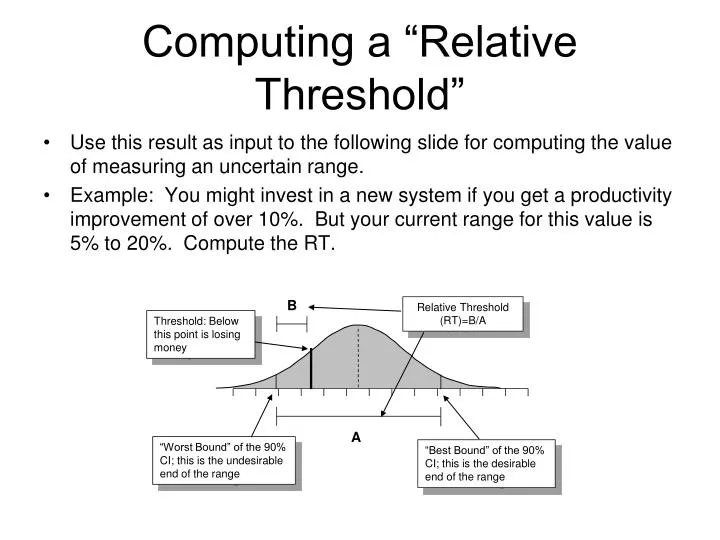
1. B Relative Threshold (RT)=B/A Threshold: Below this point is losing money A “Worst Bound” of the 90% CI; this is the undesirable end of the range “Best Bound” of the 90% CI; this is the desirable end of the range Computing a “Relative Threshold” • Use this result as input to the following slide for computing the value of measuring an uncertain range. • Example: You might invest in a new system if you get a productivity improvement of over 10%. But your current range for this value is 5% to 20%. Compute the RT.

2. Expected Opportunity Loss Factor (EOLF) 1. Compute the Relative Threshold (RT)* EOLF Curves for Uniform Distributions EOLF Curves for Normal Distributions 0.5 100 100 80 80 2. Find the RT on the vertical axis 0.4 60 60 40 40 0.3 20 0.2 20 10 10 8 3. Look directly to the right of the RT value, until you get to the appropriate curve (normal or uniform, depending on the probability distribution you are using). This is the EOLF 6 4 0.1 10 2 1 0.8 10 1 0.6 0.4 8 0.2 6 0 0.1 0.05 4 -0.1 2 4. Compute the Expected Value of Perfect Information (EVPI) = EOLF/1000*units in range*loss per unit 1 0.8 1 -0.2 0.6 0.4 -0.3 0.2 0.1 -0.4 0.08 .01 0.06 0.04 -0.5 The EOLF Chart • Use the RT from the previous slide to compute the value of information. • Example: You invested in the system in the example on the previous slide. Let’s say if the system does not get a productivity improvement greater than 10%, then you lost $100,000 for each percentage point you are under the threshold. Use this information and the RT to compute the value of reducing uncertainty about the range of potential productivity improvements.

3. Measuring to the threshold 1. Find the curve beneath the number of samples taken • Use this chart when using small samples to determine the probability that the median of a population is below a defined threshold • Example: You want to determine how much time your staff spends on one activity. You sample 12 of them and only two spend less than 1 hour a week at this activity. What is the chance that the median time all staff spend is more than 1 hour per week? Look up 12 on the top row, following the curve until it intersects the “2” line on the bottom row, and look up the number to the left. The answer is just over 1%. Number Sampled 2 4 6 8 10 12 14 16 18 20 50% 4. Find the value on the vertical axis directly left of the point identified in step 3; this value is the chance the median of the population is below the threshold 40% 30% 20% Chance the Median is Below the Threshold 10% 5% 3. Follow the curve identified in step 1 until it intersects the vertical dashed line identified in step 2. 2% 1% 0.5% 0.2% 0.1% 0 4 5 6 7 8 9 10 1 2 3 Samples Below Threshold 2. Identify the dashed line marked by the number of samples that fell below the threshold

4. Population Percentage Estimate # of Samples in subgroup 2 4 3. Repeat the process for the upper bound, using the diagonal line above the sample size; follow the diagonal line until it intersect the same vertical line as before; follow it to the number on the vertical axis to the left labeled “90% CI Upper Bound” 8% • Use this chart to estimate the percentage of a population that falls within a subgroup, given a small sample • Example: you want to measure how many of your customers have shopped at a competitor in the last week. You sample 20 and 10 of them said they did shop at a competitor. The chart shows how to compute the 90% confidence interval for the share of all customers who shopped there. 12% 16% 5 20% 10 20 15 30% 90% CI Upper Bound 1. Find the total sample size; then find the diagonal line that starts on the small circle beneath it 40% 50% 60% 70% 80% Sample Size 10 20 30 40 2 4 6 8 2 4 6 8 2 4 6 8 2 4 6 8 40% 30% 20% 10% 10 20 15 90% CI Lower Bound 8% 2. Follow the diagonal line until it intersects the vertical line that corresponds to the number of samples in the subgroup; at that point lookup the number on the vertical scale to the left labeled “90% CI Lower Bound” 6% 4% 2% 0% 2 4 6 8 # of Samples in subgroup

5. The “Enemy Tank” case • This chart shows how the WWII statisticians estimated German tank production based on serial numbers of captured tanks 100 50 1. Subtract the smallest serial number in the sample from the largest 20 10 5 2 1 Upper bound A 0.5 0.2 0.1 0.05 Mean 0.02 0.01 Lower bound 0.005 0.002 0.001 2 4 6 8 2 4 6 8 2 4 6 8 2 4 6 8 2 4 6 8 0 10 20 30 40 50 Sample Size 3. Find the value for “A” on the vertical axis closest to the point on the curve and add 1; multiply the result by the answer in step 1. This is the 90% CI UB for total serial numbered items 2. Find the sample size on the horizontal axis and follow it up to the point where the vertical line intersects the curve marked “Upper Bound” 4. Repeat steps 2 and 3 for the Mean and Lower Bound