Download
1 / 39
390 likes | 401 Views
Presented by Joseph K. Berry W. M. Keck Scholar, Department of Geography, University of Denver. GIS Modeling Week 1 — Overview GEOG 3110 –University of Denver.

E N D
Presented byJoseph K. Berry W. M. Keck Scholar, Department of Geography, University of Denver GIS ModelingWeek 1 — OverviewGEOG 3110 –University of Denver Course overview; GIS mapping, management and modeling; Discrete (map objects) vs. continuous (map surfaces); Linking data and geographic distributions; Framework for map-ematical processing
Mappinginvolves precise placement (delineation) of physical features (graphical inventory) Modelinginvolvesanalysis of spatial relationships and patterns (numerical analysis) Descriptive Mapping Prescriptive Modeling (Nanotechnology)Geotechnology(Biotechnology) Geotechnologyis one of the three "mega technologies" for the 21st century and promises to forever change how we conceptualize, utilize and visualize spatial relationships in scientific research and commercial applications (U.S. Department of Labor) Geographic Information Systems (map and analyze) Global Positioning System (location and navigation) Remote Sensing (measure and classify) GPS/GIS/RS The Spatial Triad WhereisWhat WhySo What and What If… (Berry)
Historical Setting and GIS Evolution Manual Mapping for 8,000+ years Computer Mapping…automates the cartographic process (70s) Spatial Database Management…links computer mapping with database capabilities (80s) Map Analysis…representation of relationships within and among mapped data (90s) Multimedia Mapping…full integration of GIS, Internet and visualization technologies (00s) We have been mapping for thousands of years with the primary of navigation through unfamiliar terrain and seas, with emphasis on precise placement of physical features. …but the last four decades have radically changed the very nature of maps and how they are used— Where Where is What … GIS Modeling course Why, So What and What If… Wow!!! …did you see that (Berry)
Click on… Info Tool Theme Table Distance Zoom Pan Select Theme Spatial Table Query Builder : Object ID X,Y X,Y X,Y : …identify tall aspen stands Attribute Table FeatureSpeciesetc. : : Object ID Aw : : Big …over 400,000m2 (40ha)? Discrete, irregular map features (objects) Points, Lines and Areas Descriptive Mapping Framework(Vector, Discrete) (Berry)
Hole 2)Special Punch was used to notch-out the hole assigned to a particular characteristic (attribute), such as #11 notch = Douglas fir timber type Notch #11 15 14 13 12 Where 10 9 8 7 Hole 6 Cards pulled up… … DO NOT have characteristic 5 4 3 2 Index card (tray) 1 Query Tray holds all of the index cards for a project area #57 Notch Cards falling down… … HAVE characteristic #57 Timber Stand Map (wall) 5)Card ID# identifies the timber stand polygons from the search and the appropriate locations are shaded— …a “Database-entry Geo-query” Manual GIS(Geo-query circa 1950) 1)Index Card with series of numbered holes around the edge and written description/data in the center Spatial Table (spatial objects) 3)Pass a long Needle through the stack of cards and lift… What Data Table (attribute records) 4)Repeat using the search results sub-set for more characteristics (Berry)
Click on… Shading Manager Zoom Pan Rotate Display Grid Analysis …calculate a slope map and drape on the elevation surface Continuous, regular grid cells (objects) Points, Lines, Areas and Surfaces Map Analysis Framework (Raster, Continuous) Map Stack Grid Table : --, --, --, --, --, --, --, --, --, --, --, --, --, 2438, --, --, --, --, --, : (Berry)
Course Description and Syllabus www.innovativegis.com/basis/Courses/GMcourse12/ Grading Topics and Schedule Basic Concepts Spatial Analysis GIS Modeling Spatial Statistics Future Directions (Berry)
Textbook and Companion CD-ROM Course Textbook …Required Reading …occasional in-class questions on required reading …Other Reading Online CD Materials …Further ReadingRecommended/ Optional …Text Figureslide set (color) …Optional Exercisesat end of each topic …Example Applications …MapCalcsoftware, data, tutorials and manual …Surfersoftware, sample data and tutorials …SnagIt software(recommended) Access Default.htm …to view & install materials (Berry)
Links to Class Materials(Class Webpage) Class folder in GIS lab http://www.innovativegis.com/basis/Courses/GMcourse12/ The GIS Modeling course’s main page contains links to course Administrative Materials and Readings, Lectures, and Homework assignments Links to ReadingAssignments — required readings are from the course Text with some Recommended and Optional readings on the CD and posted online Links to LectureNotes — lecture slide sets are posted Wednesdays by 5:00pm; available in the GIS Lab Thursdays by 12:00noon Links to HomeworkAssignments — exercise templates are downloaded then completed in teams and submitted to class Dropbox Links to Software — all of the software/data used in the class are on the class CD or available for download (Berry)
http://www.innovativegis.com/basis/Papers/Other/GISmodelingFramework/ Geotechnology– one of the three “mega-technologies” for the 21st Century (the other two are Nanotechnology and Biotechnology, U.S. Department of Labor) Global Positioning System(Location and Navigation) Remote Sensing(Measure and Classify) Geographic Information Systems(Map and Analyze) History/Evolution of Map Analysis 70sComputer Mapping(Automated Cartography) 80sSpatial Database Management(Mapping and Geo-query) 90sMap Analysis (Spatial Relationships and Patterns) Framework Paper Organizational Structure of this Course Spatial Analysis(Geographical context) Reclassify (single map layer; no new spatial information) Overlay (coincidence of two or more map layers; new spatial information) Proximity (simple/effective distance and connectivity; new spatial information) Neighbors (roving window summaries of local vicinity; new spatial information) Spatial Statistics(Numerical context) Surface Modeling (point data to continuous spatial distributions Spatial Data Mining (interrelationships within and among map layers) (Berry)
Traditional GIS Forest Inventory Map • Points, Lines, Polygons • Discrete Objects • Mapping and Geo-query Spatial Statistics Traditional Statistics Spatial Distribution (Surface) Minimum= 5.4 ppm Maximum= 103.0 ppm Mean= 22.4 ppm StDEV= 15.5 • Mean, StDev (Normal Curve) • Central Tendency • Typical Response (scalar) • Map of Variance (gradient) • Spatial Distribution • Numerical Spatial Relationships Mapped Data Analysis Evolution(Revolution) Spatial Analysis Elevation (Surface) • Cells, Surfaces • Continuous Geographic Space • Contextual Spatial Relationships (Berry)
Calculating Slope and Flow(map analysis) Inclination of a fitted plane to a location and its eight surrounding elevation values (Neighbors) Slope (47,64) = 33.23% Slope map draped on Elevation Slope map Flow (28,46) = 451 Paths Elevation Surface Total number of the steepest downhill paths flowing into each location (Distance) Flow map draped on Elevation (Berry) Flow map
Erosion Potential Reclassify Overlay Reclassify Erosion_potential Slopemap Slope_classes Flow/Slope Reclassify Simple Buffer Flowmap Flow_classes Protective Buffers …reach farther in areas of high erosion potential But all buffer-feet are not the same… (slope/flow Erosion_potential) Streams Simple Buffer Erosion_potential Deriving Erosion Potential & Buffers (Berry)
Distance away from the streams is a function of the erosion potential(Flow/Slope Class) with intervening heavy flow and steep slopes computed as effectively closer than simple distance— “as the crow walks” Distance Effective Erosion Distance Erosion Buffers Close Far Simple Buffer Heavy/Steep (far from stream) Erosion_potential Light/Gentle (close) Effective Buffers (digital slide show VBuff) Streams Calculating Effective Distance(variable-width buffers) (Berry)
Classes of Spatial Analysis Operators …all Spatial Analysis involves generating new map values (numbers) as a mathematical or statistical function of the values on another map layer(s) —sort of a “map-ematics” for analyzing spatial relationships and patterns— (Geographic Context) Reclassifyoperations involve reassigning map values to reflect new information about existing map features on a single map layer GIS Toolbox Overlayoperations involve characterizing the spatial coincidence of mapped data on two or more map layers (Berry)
Classes of Spatial Analysis Operators(Geographic) …all Spatial Analysis involves generating new map values (numbers) as a mathematical or statistical function of the values on another map layer(s) —sort of a “map-ematics” for analyzing spatial relationships and patterns— (Geographic Context) Proximityoperations involve measuring distance and connectivity among map locations GIS Toolbox Neighborhoodoperations involve characterizing mapped data within the vicinity of map locations (Berry)
OUR STORE …close to the store (blue) Travel-Time for Our Store to Everywhere A store’s Travelshed identifies the relative driving time from every location to the store— …analogous to a “watershed” Relative scale: 1 = .05 minutes (Berry)
Ocean Ocean Competitor 1 Competitor 2 Competitor 3 Competitor 4 Competitor 5 Ocean Ocean Ocean Travel-Time for Competitor Stores Ocean Our Store (#111) Travel-Time maps from several stores treating highway travel as four times faster than city streets. Blue tones indicate locations that are close to a store (estimated twelve minute drive or less). Customer data can be appended with travel-time distances and analyzed for spatial relationships in sales and demographic factors. (Berry)
Travel-Time Surfaces(Our Store & Competitor #4) Blue tones indicate locations that are close to a store (estimated twelve minute drive or less). Increasingly warmer tones form a bowl-like surface with larger travel-time values identifying locations that are farther away. Our Store Competitor (Berry)
Competition Map(Our Store & Competitor #4) The travel-time surfaces for two stores can be compared (subtracted) to identify the relative access advantages throughout the project area. Zero values indicate the same travel-time to both stores (equidistant travel-time) …yellow tones identifying the Combat Zone ; green Our Store advantage; red Competitor #4 advantage Competitor Our Advantage Positive Negative Our Store Competitors (See Location, Location, Location: Retail Sales Competition Analysis, www.innovativegis.com/basis/present/GW06_retail/GW06_Retail.htm) (Berry)
Mapped Data Analysis Evolution(Revolution) Exercise #1 Logistics 1) Who are we? (class photo; books; break) 2) just to make sure you are comfortable with Homework Exercises …and then on to Spatial Statistics Exercise #0 Setup (Berry)
Setting Up and Using Class Data • Moving MapCalc Data to your personal workspace • Right click on Start at the bottom left of your screen (Task Bar) • Select Windows Explorer • Locate your personal workspace as directed by the instructor (Z: drive) • Create a new folder in your workspace called …\GISmodeling • In the new folder create a sub-folder …\GISmodeling\MapCalc Data • Browse to the …\GEOG3110 class directory (I: drive) • Highlight all ofthe files/folders MapCalc Data folder on the class directory and select Copy • Go to your new …\GISmodeling\MapCalc Data sub-folder and Paste the MapCalc Data files Suggested folder organization …\GISmodeling\MapCalc Data\(…just created folder containing MapCalc base data) …\GISmodeling\Week1\(contains all of the data, scripts, screen grabs, etc. developed for week 1) …\GISmodeling\Week2\(contains all of the data, scripts, screen grabs, etc. developed for week 2) …etc. Example Exercise…download Exer0.doc to your …\GISmodeling\Week1\folder and complete under the instructor’s guidance (Berry)
Exercise #0(dry run) …in Lattice display format… …use Snagit to capture plot and paste into document Use MapCalc to generate a 3D display of the Elevation surface … …change to Grid display format… …use Snagit to capture plot and paste into document …briefly describe the differences you see between Lattice and Grid displays …email the document to me (Berry)
GIS Modeling Framework(Model Criteria) Where are the best places for a campground? …rowsrepresent Model Criteria (Berry)
Renumber Slope …map analysis operations are sequenced on map variables to implement the model’s logic Renumber Spread Analyze Renumber Spread Renumber Radiate Renumber Orient GIS Modeling Framework(Analysis Levels) “Calibration” “Algorithm” “Weighting” Modeled Interpreted Base Derived …columns represent Analysis Levels …column transitions represent Processing Approaches (Berry)
Derive (Algorithm) Gentle slopes Near roads Near water Good views Westerly Interpret (Calibrate) Combine (Weight) Mask (Constraints) Campground Suitability Model(Macro script) …the map analysis logic ingrained in the flowchart is translated into a logical series of map analysis commands(MapCalc) Tutor25_Campground Script (See “Short description of the Campground model” and “Helpful hints in Running MapCalc” in the Email Dialog section of the Class Webpage) (Berry)
Homework Exercise #1 Question #1 Model Criteria Confirm Homework Team— the class will be divided into teams containing two to three members #2 Analysis Levels Download Exercise #1— “Links to Homework,” right-click on “Exer1.doc” and choose “Save” to download …and then access the exercise in Word #3 Derived Maps #4 Calibrated Maps www.innovativegis.com/basis/Senarios/Campground.htm #5 Analyze Command Complete the exercise: #6 Masking #7 Fancy Display Due next week Thursday 5:00 pm(7 days) (…slippage possible if requested by noon) Optional Questions #1-1 and #1-2 (Berry)
Traditional GIS Forest Inventory Map • Points, Lines, Polygons • Discrete Objects • Mapping and Geo-query Spatial Statistics Traditional Statistics Spatial Distribution (Surface) Minimum= 5.4 ppm Maximum= 103.0 ppm Mean= 22.4 ppm StDEV= 15.5 • Mean, StDev (Normal Curve) • Central Tendency • Typical Response (scalar) • Map of Variance (gradient) • Spatial Distribution • Numerical Spatial Relationships Mapped Data Analysis Evolution(Revolution) Spatial Analysis Effective Distance (Surface) • Cells, Surfaces • Continuous Geographic Space • Contextual Spatial Relationships (Berry)
Classes of Spatial Statistics Operators (Spatial Statistics) …all Spatial Analysis involves generating new map values (numbers) as a mathematical or statistical function of the values on another map layer(s) —sort of a “map-ematics” for analyzing spatial relationships and patterns— (Numeric Context) GIS Toolbox Surface Modelingoperations involve creating continuous spatial distributions from point sampled data Spatial Data Miningoperations involve characterizing numerical patterns and relationships within and among mapped data (Berry)
GeoExplorationvs.GeoScience Desktop Mapping Data Space Field Data Map Analysis Geographic Space Standard Normal Curve Average = 22.0 StDev = 18.7 22.0 “Maps are numbers first, pictures later” Desktop Mappinggraphically links generalized statistics to discrete spatial objects (Points, Lines, Polygons)—non-spatial analysis (GeoExploration) X, Y, Value Point Sampled Data (Numeric Distribution) (Geographic Distribution) 40.7…not a problem Discrete Spatial Object Continuous Spatial Distribution High Pocket Spatially Generalized Spatially Detailed Discovery of sub-area… Adjacent Parcels Map Analysismap-ematically relates patterns within and among continuous spatial distributions (Map Surfaces)— spatial analysis and statistics (GeoScience) (See Beyond Mapping III, “Epilog”, Technical and Cultural Shifts in the GIS Paradigm, www.innovativegis.com/basis) (Berry)
Roving Window (count) Point Density analysis identifies the total number of customers within a specified distance of each grid location Point Density Analysis (Berry) (See Beyond Mapping III, “Epilog”, Technical and Cultural Shifts in the GIS Paradigm, www.innovativegis.com/basis)
High Customer Density pockets are identified as more than one standard deviation above the mean Unusually high customer density (>1 Stdev) Identifying Unusually High Density (See Beyond Mapping III, “Topic 26”, Spatial Data Mining in Geo-business, www.innovativegis.com/basis) (Berry)
Spatial Interpolation(Smoothing the Variability) The “iterative smoothing” process is similar to slapping a big chunk of modeler’s clay over the “data spikes,” then taking a knife and cutting away the excess to leave a continuous surface that encapsulates the peaks and valleys implied in the original field samples …repeated smoothing slowly “erodes” the data surface to a flat plane= AVERAGE (digital slide show SStat2) (Berry)
Phosphorous (P) Visualizing Spatial Relationships Geographic Distribution What spatial relationships do you SEE? …do relatively high levels of P often occur with high levels of K and N? …how often? …where? “Maps are numbers first, pictures later” Multivariate Analysis— each map layer is a continuous variable with all of the math/stat “rights, privileges and responsibilities” therewith …simply “spatially organized “ sets of numbers (matrix) (Berry)
Calculating Data Distance …an n-dimensional plot depicts the multivariate distribution— the distance between points determines the relative similarity in data patterns Pythagorean Theorem 2D Data Space: Dist = SQRT (a2 + b2) 3D Data Space: Dist = SQRT (a2 + b2 + c2) …expandable to N-space …this response pattern (high, high, medium) is the least similar point as it has thelargest data distance from the comparison point (low, low, medium) (See Beyond Mapping III, “Topic 16”, Characterizing Spatial Patterns and Relationships, www.innovativegis.com/basis) (Berry)
Clustering Maps for Data Zones Groups of “floating balls” in data space identify locations in the field with similar data patterns– data zones or Clusters …a map stack is a spatially organized set of numbers …data distances are minimized within a group (intra-cluster distance) and maximized between groups (inter-cluster distance) using an optimization procedure (See Beyond Mapping III, “Topic 7”, Linking Data Space and Geographic Space, www.innovativegis.com/basis) (Berry) (See Beyond Mapping III, “Topic 16”, Characterizing Spatial Patterns and Relationships, www.innovativegis.com/basis)
The Precision Ag Process (Fertility example) Steps 1) – 3) On-the-Fly Yield Map Map Analysis Step 4) Cyber-Farmer, Circa 1992 Farm dB Prescription Map Variable Rate Application Step 5) Step 6) As a combine moves through a field it 1) uses GPS to check its location then 2) checks the yield at that location to 3) create a continuous map of the yield variation every few feet. This map is 4) combined with soil, terrain and other maps to derive 5) a “Prescription Map” that is used to 6) adjust fertilization levels every few feet in the field (variable rate application). (Berry) (See Beyond Mapping III, “Topic 16”, Characterizing Spatial Patterns and Relationships, www.innovativegis.com/basis)
Mapped data that exhibits high spatial dependency create strong prediction functions. As in traditional statistical analysis, spatial relationships can be used to predict outcomes …the difference is that spatial statistics predicts where responses will be high or low Spatial Data Mining Precision Farming is just one example of applying spatial statistics and data mining techniques (Berry) (See Beyond Mapping III, “Topic 28”, Spatial Data Mining in Geo-business, www.innovativegis.com/basis)
Mappinginvolves precise placement (delineation) of physical features (graphical inventory) Modelinginvolvesanalysis of spatial relationships and patterns (numerical analysis) Descriptive Mapping Prescriptive Modeling (Nanotechnology)Geotechnology(Biotechnology) Geotechnologyis one of the three "mega technologies" for the 21st century and promises to forever change how we conceptualize, utilize and visualize spatial relationships in scientific research and commercial applications (U.S. Department of Labor) Geographic Information Systems (map and analyze) Global Positioning System (location and navigation) Remote Sensing (measure and classify) GPS/GIS/RS The Spatial Triad WhereisWhat WhySo What and What If (Berry)