Download
1 / 13
130 likes | 242 Views
A Comparison of Simulated Annealing and Genetic Algorithm Approaches for Cultivation Model Identification. Olympia Roeva Institute of Biophysics and Biomedical Engineering Bulgarian Academy of Sciences E-mail: olympia@clbme.bas.bg. 1. Introduction 2. Outline of the GA 4. Test problem

E N D
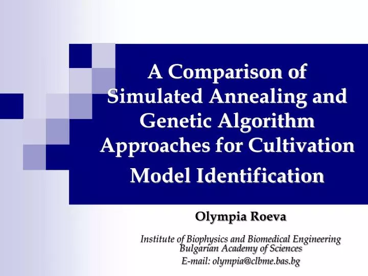
A Comparison of Simulated Annealing and Genetic Algorithm Approaches for Cultivation Model Identification Olympia Roeva Institute of Biophysics and Biomedical Engineering Bulgarian Academy of Sciences E-mail: olympia@clbme.bas.bg
1. Introduction 2. Outline of the GA 4. Test problem • 3. Outline of the SA5. Results and discussion competing paradigms in the field of modern heuristics Genetic AlgorithmSimulated Annealing Algorithm quite close relatives and much of their difference is superficial population size → one population new solutionsby → a new solution by modifying only combining two different solutionsone solution with a local move (crossover and mutation) (only mutation) In this work, both GA and SA are applied and compared for a parameter identification of non-linear mathematical model of E. coli MC4110 fed-batch cultivation process.
1. Introduction 2. Outline of the GA 4. Test problem • 3. Outline of the SA5. Results and discussion A pseudo code of a GA is presented as: 1. Set generation number to zero (t = 0) 2. Initialise usually random population of individuals (P(0)) 3. Evaluate fitness of all initial individuals of population 4. Begin major generation loop in k: 4.1. Test for termination criterion 4.2. Increase the generation number 4.3. Select a sub-population for offspring reproduction (select P(i) from P(i – 1)) 4.4. Recombine the genes of selected parents (recombine P(i)) 4.5. Perturb the mated population stochastically (mutate P(i)) 4.6. Evaluate the new fitness (evaluate P(i)) 5. End major generation loop
1. Introduction 2. Outline of the GA 4. Test problem • 3. Outline of the SA5. Results and discussion Basic GA operators and parameters
1. Introduction 2. Outline of the GA 4. Test problem • 3. Outline of the SA5. Results and discussion A pseudo code of SA could be presented as: 1. Find initial solution (by generating it randomly) 2. Set initial value for the control parameter T = T0 3. Set a value for r, the rate of cooling parameter j = 0 Generate (at random) a new solution S’ Calculate the difference in cost: = cost(S’) – cost(S) Examine the new solution and decide: accept or reject If accepted, it becomes the current solution; otherwise, keep the old one; j = j+1 Reduce the temperature and generate a new solution 4. Until some stopping criterion applies
1. Introduction 2. Outline of the GA 4. Test problem • 3. Outline of the SA5. Results and discussion Boltzman distributionwith the probability of acceptance: Temperature update:T = T0 0.95r Annealing parameters:
1. Introduction 2. Outline of the GA 4. Test problem • 3. Outline of the SA5. Results and discussion Parameter identification of E. coli MC4110 fed-batch cultivation model Real experimental data of the E. coli MC4110 fed-batch cultivationare used.
1. Introduction 2. Outline of the GA 4. Test problem • 3. Outline of the SA5. Results and discussion A two stage parameter identification procedure is used Objective function
1. Introduction 2. Outline of the GA 4. Test problem • 3. Outline of the SA5. Results and discussion
1. Introduction 2. Outline of the GA 4. Test problem • 3. Outline of the SA5. Results and discussion GA max = 0.4796, kS = 0.0162, YS/X = 2.0137 SA max = 0.4864, kS = 0.0150, YS/X = 1.9088 Table 1. Results from parameter identification – second step
Current Best Individual Best: 0.11025 Mean: 0.11602 25 150 Best fitness Mean fitness 20 100 15 Current best individual Fitness value 10 50 5 0 0 1 2 3 0 20 40 60 80 100 Number of variables (3) Generation Best, Worst, and Mean Scores Score Histogram 800 40 600 30 Number of individuals 400 20 200 10 0 0 20 40 60 80 100 0.11 0.12 0.13 0.14 0.15 Generation Score (range) • 1. Introduction 2. Outline of the GA 4. Test problem • 3. Outline of the SA5. Results and discussion Best GA result
Best point Best Function Value: 0.11041 25 25 20 20 15 15 Function value Best point 10 10 5 5 0 0 1 2 3 0 1000 2000 3000 4000 Number of variables (3) Iteration Current Point Current Function Value: 0.11207 25 40 20 30 15 Current point Function value 20 10 10 5 0 0 1 2 3 0 1000 2000 3000 4000 Number of variables (3) Iteration • 1. Introduction 2. Outline of the GA 4. Test problem • 3. Outline of the SA5. Results and discussion Best SA result
1. Introduction 2. Outline of the GA 4. Test problem • 3. Outline of the SA5. Results and discussion Cultivation of E. coli MC4110 21.2 GA model SA model 21 Exp. data 20.8 Dissolved oxygen, [%] 20.6 20.9 20.4 20.85 20.8 20.2 20.75 20.0 20.7 8.4 8.5 8.6 8.7 8.8 8.9 9 9.1 9.2 9.3 9.4 19.8 6 7 8 9 10 11 12 Time, [h]