Download
1 / 33
330 likes | 584 Views
Stochastyczny efekt Dopplera. Krzysztof Murawski UMCS Lublin. Plan. Klasyczny efekt Dopplera Trochę heliofizyki Cel badań Metoda i strategia Przesunięcia częstości fal w polach stochastycznych Gdzie jesteśmy i dokąd zmierzamy. Doppler Effect.

E N D
Stochastyczny efekt Dopplera Krzysztof Murawski UMCS Lublin
Plan • Klasyczny efekt Dopplera • Trochę heliofizyki • Cel badań • Metoda i strategia • Przesunięcia częstości fal w polach stochastycznych • Gdzie jesteśmy i dokąd zmierzamy
Doppler Effect • Change in frequency of a wave due to relative motion between source and observer. • A sound wave frequency change is noticed as a change in pitch.
Fale akustyczne w ośrodku jednorodnym Stan równowagi: =e=const., p = pe=const, Ve=0 Fale o małej amplitudzie: Ptt – cs2pxx = 0 cs2= pe/e Związek dyspersyjny 2=cs2k2 Efekt Dopplera (V 0) = cs k + Vek
Fale akustyczne w ośrodku niejednorodnym Stan równowagi: =e(x), p = pe=const, V=0 Fale o małej amplitudzie: Ptt – cs2(x)pxx = 0 Rozpraszanie – warunek Bragga ki ks = kh is =h
The Sun • Dedicated satellite measurements are allowing many of the Sun’s properties to be understood. • Most of these are restricted to measurements of the solar surface.
SOLAR B – HINODE 22.09.2006
Heliosejsmologia Oscylacje globalne
A Granule is a fountain (Stein 2007)
A hypothesis or theory is clear, decisive, and positive but it is believed by none but the man who created it. Experimental findings, on the other hand are messy, inexact things which are believed by everyone except the man who did the work. Harlow Shapley
Równania Eulera • ,t + (V) = 0 • [V,t + (V)V] =-p +g • p,t + (pV) =(1-)p V
z=(x,t) Warunki brzegowe na międzypowierzchni z=(x,t) : p1 = p2, z=(x,t) (/t + V)(-z) = 0, z =
Sound waves in simple random fields An example: A space-dependent random flow One-dimensional (/y=/z=0) equilibrium: = 0 = const ue = ur(x) pe = p0 = const
A weak random field: ur(x) = 0 The perturbation technique (e.g., Murawski & Roberts 1993) 2-c2k2 = 4k 2- E(-k) d / [2-c022] For instance, Gaussian spectrum E(k) = (2 lx /) exp(-k2lx2)
Approximate solution Expansion = c0k + 22 + 2 lx/c0 = -2/1/2 k2lx2D(2klx) - ik2lx2[1-exp(-4k2lx2)] where D()=exp(-2)0 exp(t2) dt is Dawson's integral (Press et al. 1992).
Random Gaussian mass density for its typical realization.
Fale stochastyczne Mędrek i Murawski (2002)
Numerical (asterisks, diamonds) and analytical (dashed lines) data (Murawski & Mędrek 2002)
Various random fields Sound waves in random fields: =Re r-0, a = Im r -0. <0 (>0) denotes a red (blue) shift. a<0 ( a>0) corresponds to attenuation (amplification).
Sound waves in complex fields An example: a space- and time-dependent random mass density field The dispersion relation for r(x,t): 2 - K2 = 2-- (2 E(-K,-)) d d/ (2-2) K = klx, = lx/c0
Wave noise Spectrum: E(K,)=2/ E(K) (-r(K)) Dispersionless noise: r(K) = cr K r(x,t) = r(x-crt,t=0)
Dispersion relation: 2 = K/(23/2) [cr2/(cr2-1) KD(2/c+K)] + i K2/(4) [1/c-+|c- / c+|1/c+ exp(-4K2/c+2)] c = cr 1
Real 2 Imaginary 2
Real (solid lines) and imaginary (dashed lines) parts of2 versus K for cr=-2 (left) andcr=2 (right).
Real (solid line) and imaginary (dashed line) parts of 2 for K=2. An analogy with Landau damping in plasma physics.
Conclusions • Random fields change frequencies and alter amplitudes of waves • The random p-modes problem is analogous to the random trapped waves problem • Numerical verification (Nocera et al. 2001, Murawski et al. 2001) • A number of problems remain to be solved both analytically • and numerically
Dowdy et al. (1986) Solar Phys., 105, 35 Modelling improvement Gabriel (1976), Phil. Trans. A281, 339