1 / 0

Heat Transfer

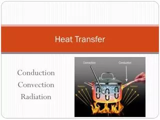
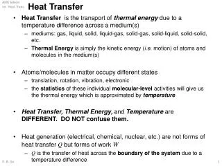
Heat Transfer. Dr. R. Velraj Professor Department of Mechanical Engineering, CEG, Anna University Chennai. Thermodynamics & Heat Transfer. Study of Heat and Work transfer (quantitatively). Thermodynamics. Study of “How heat flows”. Heat Transfer.

torn
Download Presentation

Heat Transfer

An Image/Link below is provided (as is) to download presentation Download Policy: Content on the Website is provided to you AS IS for your information and personal use and may not be sold / licensed / shared on other websites without getting consent from its author. Content is provided to you AS IS for your information and personal use only. Download presentation by click this link. While downloading, if for some reason you are not able to download a presentation, the publisher may have deleted the file from their server. During download, if you can't get a presentation, the file might be deleted by the publisher.

E N D

Presentation Transcript


  1. Heat Transfer

    Dr. R. Velraj Professor Department of Mechanical Engineering, CEG, Anna University Chennai
  2. Thermodynamics & Heat Transfer Study of Heat and Work transfer (quantitatively) Thermodynamics Study of “How heat flows” Heat Transfer every activity involves heat transfer
  3. Driving Potential & Resistance Class Room Ambience Students’ Interest & Capability Teacher’s Interest & Knowledge Knowledge Transfer Teaching – Learning Process in a Class Room RESISTANCE FACTORS Time of lecture Nature of subject Ambience (conduciveness) DRIVING POTENTIAL Difference between Teacher’s interest + knowledge & students’ interest + capability However, higher potential difference leads to increase in entropy
  4. T T T0 x Conduction The transfer of energy in a solid or fluid via molecular contact without bulk motion Solids > Lattice vibrations Fluids > Molecular collisions MODE MATHEMATICAL EQUATION PHYSICAL PHENOMENON
  5. Conduction (contd.) Fourier Law of Heat Conduction The heat flux, q is directly proportional to temperature gradient The proportionality constant, k, is defined as the thermal conductivity, a thermo physical property.
  6. Conduction (contd.) Thermal Conductivity, k Silver = 410 Wm-1K-1 k/ksilver Silver 1 Gold 0.7 Copper 0.93 Aluminum 0.86 Brass (70% Cu:30% Ni) 0.33 Platinum, Lead 0.25 Mild steel (0.1% Cu), Cast iron 0.12 Bismuth 0.07 Mercury 0.04 METALS NON-METALS k/ksilver Air 0.19 Water 0.0014 Granite, Sandstone 0.011 Average rock 0.012 Limestone 0.007 Ice 0.015 Glass (crown) 0.0058 Concrete (1:2:4) 0.0042 Brick 0.0038 Snow (fresh or average) 0.005 Soil (sandy, dry) 0.002 Soil (8% moist) 0.0033 Wood 0.0045
  7. Convection Convection occurs in liquids and gases. Energy is carried with fluid motion when convection occurs. PHYSICAL PHENOMENON MATHEMATICAL EQUATION
  8. Convection Processh(W/m2-K) Free convection Gases 2–25 Liquids 50–1000 Forced convection Gases 25–250 Liquids 50–20,000 Convection phase change 2,500–200,000 Convection (contd.) Newton’s Law of Cooling The quantity h is called the convective heat transfer coefficient (W/m2-K). It is dependent on the type of fluid flowing past the wall and the velocity distribution. Thus, h is not a thermo physical property.
  9. Convection (contd.) Convective Processes Single phase fluids (gases and liquids) Forced convection Free convection, or natural convection Mixed convection (forced plus free) Convection with phase change Boiling Condensation
  10. Radiation Energy transfer in the form of electromagnetic waves PHYSICAL PHENOMENON MATHEMATICAL EQUATION
  11. Radiation (contd.) Stefan-Boltzman Law The emissive power of a black body over all wave lengths is proportional to fourth power of temperature
  12. Heat flow out [Aq]x+Δx k Heat flow in [Aq]x g Δx One Dimensional Heat Conduction Net rate of heat gain by conduction Rate of energy generation Rate of increase of internal energy + = [Aq]x – [Aq]x+ Δx = A Δx g +
  13. Heat flow out [Aq]x+Δx k Heat flow in [Aq]x g Δx One Dimensional Heat Conduction (contd.) As Δx  0, the first term on the LHS, by definition, becomes the derivative of [Aq] with respect to x
  14. One Dimensional Heat Conduction (contd.) Rectangular Coordinates Cylindrical Coordinates Spherical Coordinates A Compact Equation n = 0 n = 1 n = 2
  15. Boundary Conditions Prescribed Temperature BC (First kind) Prescribed Heat Flux BC (Second kind) Convection BC (Third kind)
  16. Boundary Conditions Prescribed Temperature BC (First kind) Prescribed Heat Flux BC (Second kind) Convection BC (Third kind) T (x,t) | x=0 = T (0,t) = T1 T1 T2 T (x,t) | x=L = T (L,t) = T2 x 0 L
  17. Boundary Conditions Prescribed Temperature BC (First kind) Prescribed Heat Flux BC (Second kind) Convection BC (Third kind) Heat Supply Plate Conduction flux W/m2 Conduction flux Heat Supply W/m2 x 0 L
  18. Boundary Conditions Prescribed Temperature BC (First kind) Prescribed Heat Flux BC (Second kind) Convection BC (Third kind) Heat Supply Hollow Cylinder or hollow sphere W/m2 Conduction flux Heat Supply a b r W/m2 Heat Supply Conduction flux W/m2
  19. Boundary Conditions Prescribed Temperature BC (First kind) Prescribed Heat Flux BC (Second kind) Convection BC (Third kind) Convection Conduction Plate Fluid Flow Fluid Flow T1,h1 Conduction heat flux from the surface at x= 0 into the plate Convection heat flux from the fluid at T1 to the surface at x = 0 Convection Conduction T2,h2
  20. Boundary Conditions Prescribed Temperature BC (First kind) Prescribed Heat Flux BC (Second kind) Convection BC (Third kind) Convection Conduction Plate Fluid Flow Fluid Flow T1,h1 Conduction heat flux from the surface at x = L into the plate Convection heat flux from the fluid at T2 to the surface at x = L Convection Conduction T2,h2
  21. Boundary Conditions Prescribed Temperature BC (First kind) Prescribed Heat Flux BC (Second kind) Convection BC (Third kind) Fluid Flow Fluid Flow Hollow Cylinder or hollow sphere T1,h1 T2,h2 Conduction heat flux from the surface at r= a into the plate Convection heat flux from the fluid at T1 to the surface at r = a b a r Heat Supply
  22. Boundary Conditions Prescribed Temperature BC (First kind) Prescribed Heat Flux BC (Second kind) Convection BC (Third kind) Fluid Flow Fluid Flow Hollow Cylinder or hollow sphere T1,h1 T2,h2 Conduction heat flux from the surface at r= b into the plate Convection heat flux from the fluid at T2 to the surface at r = b b a r Heat Supply
  23. Steady State One Dimensional Heat Conduction Rectangular Coordinates Governing Equation 0 L x T = T1 T = T2
  24. Steady State One Dimensional Heat Conduction Cylindrical Coordinates (Solid Cylinder) Governing Equation b 0 r Solving, T = T1 T = T2
  25. Steady State One Dimensional Heat Conduction Cylindrical Coordinates (Solid Cylinder) Solved Example For r=1cm g0 = 2 x 10⁸ W/m3 k = 20 W/(m.°C) T2 = 100 °C What will be the Centre temperature T(0) Heat flux at the boundary surface (r=1cm) b 0 r Equations to use (derive) T = T1 T = T2 Solution T(0) = 350 °C q(r) = 106 W/m2
  26. Steady State One Dimensional Heat Conduction Determination of Temperature Distribution Cylindrical Coordinates (Hollow Cylinder) Mathematical formulation of this problem is k in a < r < b b Solving, T2 a T1 0 r
  27. Steady State One Dimensional Heat Conduction Expression for radial heat flow Q over a length H Cylindrical Coordinates (Hollow Cylinder) The heat flow is determined from, k Since, b T2 a T1 Rearranging, 0 r where,
  28. Steady State One Dimensional Heat Conduction Expression for thermal resistance for length H Cylindrical Coordinates (Hollow Cylinder) k Above equation can be rearranged as, b T2 where, a T1 0 here, A0 = 2πaH =area of inner surface of cylinder A1 = 2πbH =area of outer surface of cylinder Am = logarithmic mean area t = b – a = thickness of cylinder r
  29. Steady State One Dimensional Heat Conduction Expression for temperature distribution Spherical Coordinates (Hollow Sphere) The mathematical formulation is given by, in a < r < b a r 0 where, b
  30. Steady State One Dimensional Heat Conduction Expression for heat flow rate Q and thermal resistance R Spherical Coordinates (Hollow Sphere) Heat flow rate is determined using the equation, a r 0 using, from last slide b where,
  31. Composite Medium Example (Furnace Wall) FURNACE REFRACTORY LINING 1 REFRACTORY LINING 2 Ambient BRICK WALL FURNACE WALL
  32. Composite Medium Example (Condenser Water Tube) Condensing Medium (Steam) Tube Wall Scale Cooling Water
  33. Composite Medium Composite Slab (resistance in series) L1 L2 L3 Ta Q T0 Q T1 Tb T2 T3 Fluid Flow Fluid Flow Tb,hb Ta,ha Tb T1 T3 Ta T0 T2 Q Q Rb R3 R1 R2 Ra
  34. Composite Medium Composite Slab (resistance in parallel) Insulated A B E C T1 T2 D Insulated T2 T1 RE RB RA Rc RD
  35. Composite Medium Composite Cylinder H k2 k3 k1 ha hb Tb T1 T3 Ta T0 T2 Q Q Rb R3 R1 R2 Ra
  36. Composite Medium Composite Spheres ha k1 k3 k2 Tb T1 T3 Ta T0 T2 Q hb Q Rb R3 R1 R2 Ra
  37. Composite Medium Critical Thickness of Insulation H Convection into an ambient at T∞,h0 Heat Loss, q r1 T1 ro rc Insulation Radius, r
  38. Composite Medium Critical Thickness of Insulation The rate of heat loss Q from the tube is given by Convection into an ambient at T∞,h0 H r1 T1 ro For Cylinder For Sphere
  39. Composite Medium Solved Example (Composite Cylinder) Calculate, Heat loss from tube for length H=10m Temperature drops resulting in thermal resistances 7.6 cm 5 cm Determination of heat loss Ta=330°C ha=400 W/(m2.°C) Insulation t =2 cm K=0.2 W(m.°C) K = 15 W/(m °C) Ambient air Tb=30°C hb= 60 W/(m2.°C)
  40. Composite Medium Solved Example (Composite Cylinder) Calculate, Heat loss from tube for length H=10m Temperature drops resulting in thermal resistances 7.6 cm 5 cm Determination of heat loss Ta=330°C ha=400 W/(m2.°C) Insulation t =2 cm K=0.2 W(m.°C) K = 15 W/(m °C) Ambient air Tb=30°C hb= 60 W/(m2.°C)
  41. Composite Medium Solved Example (Composite Cylinder) Calculate, Heat loss from tube for length H=10m Temperature drops resulting in thermal resistances 7.6 cm 5 cm Determination of temperature drops Ta=330°C ha=400 W/(m2.°C) Insulation t =2 cm K=0.2 W(m.°C) K = 15 W/(m °C) Ambient air Tb=30°C hb= 60 W/(m2.°C)
  42. GYPSUM SHEATH Outside Air Convection h=15 W/m2 C 8cm k=0.96 1.9cm k=0.48 1.9cm 40.6 cm Inside Air Convection h=7.5 W/m2 C 2x 4 STUDS Composite Medium Solved Example (Composite Wall) 2 x 4 wood studs have actual dimensions of 4.13 x 9.21 cm with k = 0.1 W/m.°C Calculate, Overall heat transfer coefficient R value of the wall COMMON BRICK, k =0.69 Thermal resistance model INSULATION, k=0.04 Two parallel heat flow paths are possible Through the studs Through the insulation Rsheath outside Rsheath inside Rinsul Tair inside Rbrick Tair outside Rconvection inside Rconvection outside Rsheath outside Rsheath inside Rstud Note: ‘k’ is expressed in W/m °C
  43. GYPSUM SHEATH Outside Air Convection h=15 W/m2 C 8cm k=0.96 1.9cm k=0.48 1.9cm 40.6 cm Inside Air Convection h=7.5 W/m2 C 2x 4 STUDS Composite Medium Solved Example (Composite Wall) Calculate, Overall heat transfer coefficient R value of the wall COMMON BRICK, k =0.69 Heat flow through the studs Area = 0.0413m2/unit depth Heat flow occurs through 6 thermal resistances Convection Resistance outside of brick Conduction resistance in brick Conduction resistance through outer sheet Conduction resistance through wood stud Conduction resistance through inner sheet Convection resistance on inside Recall, INSULATION, k=0.04 Note: ‘k’ is expressed in W/m °C
  44. GYPSUM SHEATH Outside Air Convection h=15 W/m2 C 8cm k=0.96 1.9cm k=0.48 1.9cm 40.6 cm Inside Air Convection h=7.5 W/m2 C 2x 4 STUDS Composite Medium Solved Example (Composite Wall) Calculate, Overall heat transfer coefficient R value of the wall COMMON BRICK, k =0.69 Heat flow through the insulation INSULATION, k=0.04 The five of the materials are same, but the resistances involve different area terms, i.e., 40.6 - 4.13 cm instead of 4.13 cm. Thus the total resistance of the insulation section is given below Note: ‘k’ is expressed in W/m °C
  45. GYPSUM SHEATH Outside Air Convection h=15 W/m2 C 8cm k=0.96 1.9cm k=0.48 1.9cm 40.6 cm Inside Air Convection h=7.5 W/m2 C 2x 4 STUDS Composite Medium Solved Example (Composite Wall) Calculate, Overall heat transfer coefficient R value of the wall COMMON BRICK, k =0.69 1. Overall heat transfer coefficient Overall resistance is obtained by combining the parallel resistances as calculated earlier. Overall heat transfer coefficient is found by, (here, A = 0.406m2) INSULATION, k=0.04 Note: ‘k’ is expressed in W/m °C
  46. GYPSUM SHEATH Outside Air Convection h=15 W/m2 C 8cm k=0.96 1.9cm k=0.48 1.9cm 40.6 cm Inside Air Convection h=7.5 W/m2 C 2x 4 STUDS Composite Medium Solved Example (Composite Wall) Calculate, Overall heat transfer coefficient R value of the wall COMMON BRICK, k =0.69 2. R Value of the wall The resistance of the wall is calculated using the overall heat transfer coefficient, as given below: INSULATION, k=0.04 Note: ‘k’ is expressed in W/m °C
  47. Composite Medium Solved Example (Critical Thickness of Insulation) Calculate, the critical thickness of rubber and the maximum heat transfer rate per metre length of conductor. The temperature of rubber is not to exceed 65 °C (due to heat generated within). Ambient at 30°C, 8.5 W/m2K Critical thickness r = 5mm Maximum heat transfer rate Rubber k = 0.155 W/mK
  48. q = heat generated per unit volume x=0 Tw x Tw L L Heat Source Systems Plane wall with heat generation Expression for mid plane temperature is given by, The temperature distribution can also be written in alternative form as:
  49. Conduction-Convection Systems Internal Conductive resistance Surface Convective resistance Fins / Extended Surfaces Necessity for fins Biot Number = FIN TYPES LONGITUDINAL RECTANGULAR FIN RADIAL FIN
  50. Conduction-Convection Systems Governing Equation (Rectangular Fin) Net Heat Conducted – Heat Convected = 0 t A qx qx+dx base x dx Z L where, &
  51. Conduction-Convection Systems Boundary Conditions LONG FIN SHORT FIN (end insulated) SHORT FIN ( end not insulated)
  52. Conduction-Convection Systems Types of Fin Boundaries * For higher values of mL (i.e., m=4), tanh mL = 0.999 ≈ 1. Thus Qshort fin  Qlong fin for higher values of mL
  53. Conduction-Convection Systems Performance Parameters Fin Efficiency In practical applications, a finned heat transfer surface is composed of the finnedsurfaces and the unfinned portion. In such cases total heat transfer is used. Qtotal= Qfin + Qunfinned = ηafh θ0 + ( a – af) h θ0 Where, a = total heat transfer area (i.e., fin surface + unfinned surface) af= heat transfer area of fins only Qtotal = [ηβ+(1-β)] a h θ0 ≡ η‘ a h θ0 Where, η‘ = βη +1 – β = area – weighted fin efficiency β = af / a
  54. Conduction-Convection Systems Performance Parameters Fin Efficiency Each curve is specific for specific fin configuration Fin Efficiency, η L (2h/kt)0.5 Fin efficiency curves are available for fins of various configuration (eg. Axial, circular disk fins of various length, thickness etc)
  55. Conduction-Convection Systems Performance Parameters Fin Effectiveness Although the addition of fins on a surface increases surface area, it also increases thermal resistance over the portion of the surface where fins are attached. Therefore there may be situations in which the addition of fins does not improve heat transfer. Pk / (Ah) > 1 (to justify usage of fins)
  56. Conduction-Convection Systems Solved Example A steel rod is exposed to ambient air. If one end of the rod is maintained at a temperature of 120°C, calculate the heat loss from the rod The condition for other end of the rod is not specified explicitly. By considering L/D ratio, it appears that a long fin assumption is applicable. Using the simplest analysis to solve, computing mL: Therefore, expression for Qlong fin can be used. Diameter = 2cm Length = 25 cm k = 50 W / m. °C Tbase=120°C Tamb= 20°C h = 64 W / m2. °C
  57. Conduction-Convection Systems Solved Example (Fin Efficiency) Circular disk fins of constant thickness are attached on a 2.5 cm OD tube with a spacing of 100 fins per 1m length of tube. Fin Properties: Aluminium k = 160 W / m.°C, t = 1mm L = 1 cm Tube wall temperature = 170 °C; Ambient temperature = 30 °C Heat transfer coeff. of ambient , h = 200 W/m2. °C. Calculate, Fin Efficiency and area weighted fin efficiency Heat lost to the ambient air per 1m length of tube Heat loss with that if there were no fins on tube L t Fin Efficiency, η CIRCULAR DISK FIN Fin Efficiency Fin efficiency is determined using the graph shown aside. The following parameters are calculated, firstly: ro/ri L (2h/kt)0.5
  58. Conduction-Convection Systems Solved Example (Fin Efficiency) Calculate, Fin Efficiency and area weighted fin efficiency Heat lost to the ambient air per 1m length of tube Heat loss with that if there were no fins on tube L Area Weighted Fin Efficiency t Ratio of heat transfer area for fin to the total heat transfer area, β Fin Surface per cm of tube length = 2π(r02-ri2) = 2π[2.252-1.252] = 21.99 cm2 Total heat transfer surface per cm of tube length = 2π (r02-ri2) + 2πri (1 – t) = 2π[2.252-1.252] + 2π(1.25)(1 – 0.1) = 29.06 cm2 β = af / a = 21.99 / 29.06 = 0.757 Area Weighted Fin Efficiency, η’ = βη +1 – β = 0.757(0.9) + 0.243 = 0.924 CIRCULAR DISK FIN Tube OD = 2.5 cm 100 fins per 1m tube length kfin = 160 W/m°C t = 1mm; L = 1cm Ttube = 170°C; Tamb = 30°C hamb = 200 W/m2. °C
  59. Conduction-Convection Systems Solved Example (Fin Efficiency) Calculate, Fin Efficiency and area weighted fin efficiency Heat lost to the ambient air per 1m length of tube Heat loss with that if there were no fins on tube L Heat lost to ambient per 1m length of tube t Total heat transfer surface a per 1m of tube length a = 29.06 x 100 cm2 = 0.29 m2 Q = η’ahθ0 = 0.924 x 0.29 x 200 (170 – 30) = 7503 W CIRCULAR DISK FIN Tube OD = 2.5 cm 100 fins per 1m tube length kfin = 160 W/m°C t = 1mm; L = 1cm Ttube = 170°C; Tamb = 30°C hamb = 200 W/m2. °C Heat lost per 1m length of tube with no fins Qno fin = 2πrihθ0 = 2π x 0.0125 x 200 x (170 – 30) = 2199 W Clearly, the addition of fins increases the heat dissipation by a factor of about 3.4
  60. Transient Conduction If the surface temperature of a solid body is suddenly altered, the temperature within the body begins to change over time. Variation of temperature both with position and time makes determination of temperature distribution under transient condition more complicated. In some situations, variation of temperature with position is negligible under transient state, hence the temperature is considered to vary only with time. The analysis under the above assumption is called lumped system analysis. Biot Number, Bi = (hx) / k Lumped System Analysis is applicable only when Bi < 0.1
  61. Systems with Negligible Internal Resistance Lumped Heat Analysis The convective heat loss from the body (shown aside) has its magnitude equal to decrease in internal energy of solid. On Integration, Solving and rearranging, Q Volume V Area A S T∞ T0 T T=T0 at t=0 1/hA Cth=ρcV T∞
  62. Systems with Negligible Internal Resistance Biot Number It is a non-dimensional parameter used to test the validity of the lumped heat capacity approach. The characteristic length (Lc) for some common shapes is given below: Plane Wall (thickness 2L)Long cylinder (radius R) Sphere (radius R) Cube (side L) The lumped heat capacity approach for simple shapes such as plates, cylinders, spheres and cubes can be used if Bi < 0.1
  63. Systems with Negligible Internal Resistance Response time of a Temperature measuring Instrument For a rapid response of temperature measuring device, the index, (hAt/ρcV) should be large to make the exponential term reach zero faster. This can be achieved by decreasing wire diameter, density and specific heat or by increasing value of ‘h’. The quantity (ρcV/hA) has the units of time and is called ‘time constant’ of system. Hence at time t=t* (one time constant), At the end of time period t* the temperature difference between the body and ambient would be 0.368 of the initial temperature difference. In other words, the temperature difference would be reduced by 63.2 percent. This reduction in 63.2 percent of initial temperature difference is called ‘sensitivity’ Lower the value of time constant, better the response of instrument.
  64. Systems with Negligible Surface Resistance When convective heat transfer coefficient at the surface is assumed to be infinite, the surface temperature remains constant at all the time (t>0) and its value is equal to that of ambient temperature. The systems exhibiting above said conditions are considered to have ‘negligible surface resistance’ An important application of this process is in heat treatment of metals by quenching, viz., the dropping of a metallic sphere initially at 300 °C into a 20 °C oil bath. Mathematical formulation of this case is : T0(x) for t = 0 Ts = T∞ (t>0) Ts Large Flat Plate with Negligible Surface Resistance x L Boundary Conditions
  65. Heat flow in an Infinitely Thick Plate Semi-infinite body A semi-infinite body is one in which at any instant of time there is always a point where the effect of heating / cooling at one of its boundaries is not felt at all. At this point the temperature remains unchanged. Mathematical formulation is : with initial and boundary conditions, Ts at t=0 Qo To x Semi-Infinite Plate
  66. Systems with Finite Surface and Internal Resistance Mathematical formulation : h h T∞ T∞ at t=0 -x Infinitely Large Flat Plate of Finite Thickness (2L) x x=-L x=0 x=L
  67. Chart Solutions of Transient Heat Conduction Problems Heisler Charts (by Heisler, 1947) Infinite Plate hL/k T(x,t) - T∞ Ti- T∞ Time History Mid Plane 0.1 0.2 0.4 0.5 0.6 0.8 0.9 1 Fourier number, ατ/L2
  68. Chart Solutions of Transient Heat Conduction Problems Heisler Charts (by Heisler, 1947) Infinite Plate 1 x/L 0.2 0.4 T(x,t) - T∞ Ti- T∞ 0.6 Time History Any Position, x 0.8 0.9 1 0 0.1 100 Biot Number, hL/k
  69. Chart Solutions of Transient Heat Conduction Problems Heisler Charts (by Heisler, 1947) Infinite Plate hL/k 1 0.1 10 0.001 50 0.5 0.05 20 40 0.01 Q/Qo Heat Flow
  70. Lumped System Analysis Solved Example Determination of Time required to cool Volume 5.5 kg Aluminium Ball ρ = 2700 kg/m3 c = 900 J/kg K k = 205 W/mK Radius Tinitial=290°C Characteristic Length Tfluid = 15°C h = 58 W / m2. °C ? Time required to cool the aluminium ball to 95°C
  71. Lumped System Analysis Temperature Measurement by Thermocouples Solved Example The temperature of a gas stream is to be measured by a thermocouple whose junction can be approximated as a 1mm diameter sphere (shown aside) Determine how long it will take for the thermocouple to read 99% of initial temperature difference Thermocouple Wire Lc = V/As = (1/6)D = (1/6)x0.001 = 1.67x10⁻⁴ m Bi = hL/k = (210x 1.67x10-4) x 35 = 0.001 < 0.1 Therefore, lumped system analysis is applicable. In order to read 99% of initial temperature difference Ti – T∞ between the junction and the gas, we must have Gas T∞ h=210 W/m2 °C Junction (Sphere) D= 1mm ρ = 8500 kg/m3 k = 35 W/mK c = 320 J/kg K How long will it take for the thermocouple to read 99 % of Initial Temperature difference ?
  72. Lumped System Analysis Temperature Measurement by Thermocouples Solved Example The temperature of a gas stream is to be measured by a thermocouple whose junction can be approximated as a 1mm diameter sphere (shown aside) Determine how long it will take for the thermocouple to read 99% of initial temperature difference Thermocouple Wire Time Gas T∞ h=210 W/m2 °C Junction (Sphere) D= 1mm ρ = 8500 kg/m3 k = 35 W/mK c = 320 J/kg K How long will it take for the thermocouple to read 99 % of Initial Temperature difference ? t = 10s
  73. Transient Conduction in Semi-infinite Solids Solved Example A water pipe is to be buried in soil at sufficient depth from the surface to prevent freezing in winter. What minimum depth is required to prevent the freezing of pipe when soil is at uniform temperature of Ti = 10 °C, the surface is subjected to a uniform temperature of T0 = -15 °C continuously for 50 days. Also the pipe surface temperature should not fall below 0 °C
  74. Transient Conduction in Semi-infinite Solids Solved Example Water Pipe (to be buried) Tsurface = -15 °C SOIL ? Tsoil = 10 °C Condition : Tpipewall should not fall below 0 °C What burial depth is needed to prevent freezing of the pipe ?
  75. Temperature Distribution in Semi-infinite Solid T(x,t) - Tsurface Tinitial- Tsurface
  76. Determination of Burial depth
  77. Determination of Burial depth The pipe should be buried at least to a depth of 1.12 m to prevent freezing.
  78. Application of Heisler Charts Aluminium Slab Thickness=10cm α = 8.4x10⁻⁵ m2/s ρ = 2700 kg/m3 c = 900 J/kg K k = 215 W/mK Tinitial=500°C Tfluid = 100°C h = 1200 W / m2. °C Mid-plane Temperature and Surface Temperature after 1 min?
  79. Determination of Mid plane Temperature 2L=10 cm ; L = 5 cm ; t = 1min = 60 s αt/L2 = (8.4x10-5 x 60) / 0.052 = 2.016 Bi = hL/k = (1200x0.05) x 215 = 0.28 Using above two parameters in Heisler Chart,
  80. Determination of Surface Temperature For x/L = 1 and Bi = 0.28,
  81. Energy Loss h2αt/k2 = (12002x8.4x10-5 x 60) / 2152 = 0.157 Bi = hL/k = (1200x0.05) x 215 = 0.28 Using above 2 parameters in Heisler Chart for Heat flow, Q/Q0 = 0.32
  82. Heat removed per unit surface area
More Related