Download
1 / 25
270 likes | 513 Views
Square Root Function- The Restoring Algorithm. VLSI–Lab project Moran Amir Elior. Goals and needs . The squaring function performs the basic math operation f(A) = Q such that Q 2 = A.

E N D
Square Root Function- The Restoring Algorithm VLSI–Lab project Moran Amir Elior
Goals and needs • The squaring function performs the basic math operation f(A) = Q such that Q2 = A. • The root method is considered difficult to implement in hardware, and requires iterative process (or use of lookup table). • We present a method which is accurate (not an approximation). The results are Q and R such that:
Motivation • The restoring method is based on “binary” search over the result range of the input, which is half the input bits. • Each time, the last remainder is sign checked. • If the remainder >= 0, we search in the upper domain, else, the lower domain. • Since this is a square root, we can divide the input by 4 and not by 2.
The Restoring Algorithm • Initial conditions: > Let R (the remainder) equal A, the input. > Let Q equal 0. Q =q1… qn • Iterative step (i is the index): > if R>>2i >= { Q , 0 ,1 } then qj-1 = ‘1’ ; R = R – {Q , 0 , 1} > if R>>2i < { Q , 0 ,1 } then qj-1 = ‘0’ ; R = R R and Q are best thought of as changing in width, bit wise; in reality, they will be zero padded from the left. We Compare R, which is originally the input, to the main terms of the square of q (as was explained for the squaring function method): 26a3 , 24a2 , 22 a1, 20a0 (4 bit example) If we are bigger, we add zero to the result and keep the remainder; if we are smaller or equal we add one to the result, and subtract the term from the remainder such that we are left with the minor terms.
Implementation issues • The operations needed are: > Subtraction > Shifting • We can use a simple Data-path for this operators. • We can use multiplied Conditional Subtraction (SC) units as well. • For each of them, there are n/2+1 iterations.
Behavioral VHDL designFor Data Path implementation • Qj := "00000000"; • R2j := D; • FOR j IN 4 DOWNTO 1 LOOP • Shift8(Qj,j,'1',Q_t); • Q_t(j+j-2) := '1'; • Subtract(R2j,Q_t, R_t, negative); • IF (negative = '0') THEN • Qj(j-1) := '1'; • R2j := R_t; • ELSE • Qj(j-1) := '0'; • END IF; • END LOOP;
Using a Data path 0 Q R load 1 0 1 ALU sign
Design reuse: ALU already exists. Simplicity: SC units are easy to implement: procedure SC ( signal CO, S : out Std_Logic ; signal R, D, CI, Q : in Std_Logic ) is begin CO <= (R and D) or (R and CI) or (D and CI) ; S <= R xor ((D xor CI) and Q) ; end SC ; Area: ~ same as ALU. Speed: ALU demands 4-5 cycles. The SC units can produce output much faster. Power: Lower than ALU ALU iteration number: q iteration SC unit count: 0.5*q2 +2.5*q - 1 Considerations
A 0 1 2 3 4 5 6 7 Q 0 0 1 1 1 2 2 2 R 0 0 0 1 2 0 1 2 Results on Schematics
Results on Schematics II A 8 9 10 11 12 13 14 15 Q 0 2 3 3 3 3 3 3 R 0 4 0 1 2 3 4 5
The SC unit maximal delay Few transients with the maximal delays 1.62nS SC max latency
On 25 cycles Power The most power consuming cycle is marked in red. 25mW RMS
Transistor count & latency • The SC unit: 34 MOS devices SC max latency ~ 2.5nSec (includes margin) • The Square Root extractor: 17 SC units 17 * 34 = 578 MOS devices Circuit max latency – 15XSC Latency = 40nSec Max working frequency = 25MHz RMS power on most consuming cycle = 25mW Highest power peek measured = 1W
Performance evaluation • Using ALU scheme will require minimum of 4 cycles => 400 nSec • Circuit improves speed by a factor of 10. • Area is not much less than the ALU unit itself excluding the peripheries we should have add.
Credits for pictures • Alain Guyot’s site for TIMA Laboratory • http://tima-cmp.imag.fr/~guyot/Cours/Oparithm/english/Extrac.htm