Canadian Centre for Climate Modelling and Analysis (CCCma) Victoria, BC Canada

1. Environment Canada's Seasonal to Multi-Seasonal Forecasts: Formulation and Interpretation Bill Merryfield Canadian Centre for Climate Modelling and Analysis (CCCma) Victoria, BC Canada Ouranos Workshop , 3 Sep 2014

2. Topics discussed • The nature of seasonal forecasting • Environment Canada’s Canadian Seasonal to Interannual Prediction System (CanSIPS): Models and initialization • Processing of model forecast data • Interpretation of EC seasonal forecast products • CanSIPS research and development

3. Nature of seasonal forecasting

4. Predictability and Prediction

5. Forecasts must communicate uncertainty Guiding principles of climate (e.g. seasonal) forecasting Probabilities ensemble forecasts • Forecasts should be interpreted in the context of past performance (skill) many years of hindcasts

6. Probabilistic forecast Seasonal mean temperature Here the forecast probability distribution or PDF is described in terms of probabilities that forecast seasonal mean temperature will fall into climatologically equi-probable tercile categories: below normal near normal above normal

7. Forecast lead Forecast issued f= forecast anomaly o= observed anomaly Some terminology Lead 0 months Forecast valid Lead 1 month Perfect _ 1 • Skill scores Example: Anomaly correlation fo AC= No skill _ (f) (o) 0 (?) _ -1 f’ f’ f’ AC=0.9 AC=0.5 AC=0.3 o’ o’ o’

8. The phenomenon being forecast must be potentiallypredictable • Prediction method being used must be able to capitalize on this potential predictability Necessary conditions for useful climate predictions

9. Seasonal forecasting methods • Earliest standard: empirical/statistical forecasts - based on historically observed relations between predictors and lagged predictand - subject to data limitations, artificial apparent skill due to “selective predictors” phenomenon - typically deterministic only • Later standard: two-tier model ensemble forecasts - model sea surface temperature (SST) prescribed - used by EC from 1995 until 2011 (anomaly persistence SST) - forecast range limited to 4 months • Current standard: coupled climate model ensemble forecasts - fully interactive atmosphere/ocean/land/(sea ice) - SSTs predicted as part of forecast - potentially useful forecast range greatly extended

10. Observed SST anomaly … “Forecast” (persisted) SST anomaly Motivation for coupled vs2-tier system Mar 2006 Apr 2006 (lead 0) Example: consider 2-tier forecast (persisted SSTA) from 1 April 2006 May 2006 (lead 1) Jun 2006 (lead 2) Jul 2006 (lead 3) 2-tier system with persisted SSTA cannot predict an El Niño or La Niña Oct 2006 (lead 6)

11. WMO Global Producing Centres for Long Range Forecasts coupled (interactive atmosphere + ocean) 2-tier (atmosphere + specified ocean temps)

12. Operational Multi-Seasonal Forecast Ranges M O A F J M J A F M A A M J M F J A J J M J J J A J M A M S O M J J A N M F M A F M F A A M J J M S M A M A J S A N O J J D J M M A Example: 1 January start Lead (months) ECMWF System 4 0 1 2 3 4 7 months NCEP CFSv2 0 1 2 3 4 5 6 9 months 0 CMC CanSIPS 1 2 3 4 5 6 7 8 9 12 months

13. Formulation: Models and initialization

14. The Canadian Seasonal to Interannual Prediction System (CanSIPS) • Developed at CCCma • Operational at CMC since Dec 2011 • 2 models CanCM3/4, 10 ensemble members each • Hindcast verification period = 1981-2010 • Forecast range = 12 months • Forecasts initialized at the start of every month

15. CanSIPS Models CanAM4Atmospheric model - T63/L35 (2.8 spectral grid) - Deep conv as in CanCM3 - Shallow conv as per von Salzen & McFarlane (2002) - Improved radiation, aerosols CanAM3Atmospheric model - T63/L31 (2.8 spectral grid) - Deep convection scheme of Zhang & McFarlane (1995) - No shallow conv scheme - Also called AGCM3 CanOM4 Ocean model - 1.41°0.94°L40 - GM stirring, aniso visc - KPP+tidal mixing - Subsurface solar heating climatological chlorophyll SST bias vs obs (OISST 1982-2009) C C

16. Modeled ENSO Teleconnections DJF Regressions against Nino3.4 index (plotted where correlation>0.3) Contours = Sea Level Pressure Merryfield et al. (MWR 2013)

17. Atmospheric assimilation SST nudging Sea ice nudging Ensemble member assimilation runs forecasts CanSIPS initialization

18. Data Sources: Hindcasts vs Operational

19. Impacts of AGCM assimilation: Improved land initialization Correlation of assimilation run vs Guelph offline analysis SST nudging only SST nudging + AGCM assim Soil temperature (top layer) Soil moisture (top layer)

20. 21 Jan 2014 1 Feb 2014 Probabilistic soil moisture forecast Feb 2014 lead 0 9 Feb 2014 Evidence CanSIPS soil moisture initialization is somewhat realistic 28 Feb 2014 25 Feb 2014

21. Skill enhancement attributable to realistic land initial conditions(soil moisture) Left to right: increased initial soil moisture anomalies • 10 models including CanCM3 • 100 start dates in warm months 1986-1995 Koster et al. GRL 2010 Less skill More skill

22. Formulation: Processing of model output

23. Correction for model biases • Because climate models are imperfect, each model has its own climate that differs from that of the real world • Thus, models initialized near observed climate state will progressively drift towards biased model climate: • These biases can be factored out by computing anomalies with respect to forecast climatology that is a function of forecast time and lead time, & comparing with observed anomalies time obs climatology forecast climatology model climatology

24. Correction for model biases (cont.) • Observed anomalies: • Forecast anomalies: where < > indicates averaging over some standard set of years (e.g. 1981-2010) O(tforecast,yi) = O (tforecast,yi) - <O (tforecast,yi)> F(tforecast,tlead,yi) = F (tforecast, tlead,yi) - <F (tforecast, tlead,yi)>

25. CanSIPS model temperature biases Biases of freely running models relative to ERA-Interim reanalysis 1981-2010 Merryfield et al. (MWR 2013)

26. CanSIPS model precipitation biases Biases of freely running models relative to GPCP2.1 1981-2010 DJF JJA Merryfield et al. (MWR 2013)

27. Construction of PDF Example: lead 0 SON 2014 temperature forecast for Montreal Anomalies for each ensemble member Gaussian fit Calibrated PDF 70% prob above normal 85% prob above normal 76% prob above normal Calibration: From hindcasts, find optimal rescaling of Gaussian mean and  that maximizes probabilistic skill score Details: Kharin et al. (A.-O., 2009)

28. Interpretation of forecasts

29. Advantages of calibrated probability forecasts Temperature • uncalibrated probabilities: - high probabilities predicted far more frequently than observed - overconfident, especially for precipitation and near- normal category - near-normal grossly overpredicted • calibrated probabilities: - much more reliable (forecast probability  observed frequency) - less overconfident - near-normal less overpredicted uncalibrated calibrated perfect forecast Brier skill score = 0 no resolution

30. Advantages of calibrated probability forecasts Precipitation • uncalibrated probabilities: - high probabilities predicted far more frequently than observed - overconfident, especially for precipitation and near- normal category - near-normal grossly overpredicted • calibrated probabilities: - much more reliable (forecast probability  observed frequency) - less overconfident - near-normal less overpredicted uncalibrated calibrated perfect forecast Brier skill score = 0 no resolution

31. CanSIPS ENSO prediction skill OISST obs lead 0 … lead 9 Nino3.4 anomaly correlation skill: 0.55 < AC < 0.84 at 9-month lead Does this translate to long lead skill over Canada?

32. Canada 2m temperature skill at 9 month lead Anomaly Correlation Long-lead skill for western Canada in winter/spring JFM FMA MAM Long-lead skill for eastern Canada in summer/fall JAS ASO SON

33. Global precipitation skill at 9 month lead Anomaly Correlation NDJ DJF JFM

34. Canada precipitation skill at 1 month lead Anomaly Correlation JFM FMA MAM JAS ASO SON

35. CanSIPS soil moisture forecasts & skill JJA 2011 (lead 0) 3-category probabilistic forecast (left)  ERA-interim verification (right)  Anomaly correlation* JJA (lead 0) Soil moisture (left)  2m temperature (right)  SM T2m *ERA-interim verification

36. Evidence that CanSIPS snow initialization is somewhat realistic Example: BERMS Old Jack Pine Site (Saskatchewan) CanCM3 assimilation runs CanCM4 assimilation runs 2002-2003 1997-2007 climatology vs in situ obs

37. CanSIPS snow water equivalent (SWE) forecasts & skill JFM 2012 (lead 0) 3-category probabilistic forecast (left)  MERRA verification (right)  Anomaly correlation JFM (lead 0) SWE (left)  2m temperature (right)  • Higher than for T2m • in snowy regions! SWE T2m

38. Mean anomaly correlations over Canada vs predicted season & lead Near-surface temperature Precipitation lead 0 months lead 1 month lead 2 months lead 3 months Soil moisture Snow water equivalent

39. Additional deterministic and probabilistic skill scores SON temperature (lead 0 months)

40. Additional deterministic and probabilistic skill scores SON precipitation (lead 0 months)

41. Towards CanSIPSv2

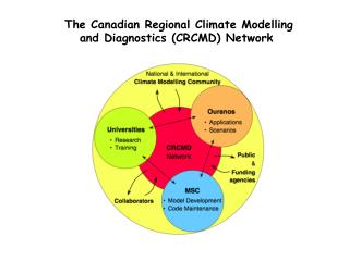
42. Improved ocean initialization Improved sea ice initialization Improved land initialization based on EC’s Canadian Land Data Assimilation System (CaLDAS) Improved climate model components (atmosphere, ocean, land, sea ice) New coupled model based on MSC’s GEM weather prediction model Regional downscaling of global model forecasts? CanSIPS Development Efforts

43. Experimental downscaling of CanSIPS forecasts • CanRCM4 = Canadian Regional Climate Model version 4 • CORDEX North America grid – 0.22 ~ 25 km resolution • RCM runs will be initialized from downscaled assimilation runs • Can be run concurrently with global forecasts • Potential to become operational if added value demonstrated Soil moisture probabilistic forecast on CanSIPS global grid Surface temperature on CanRCM4 0.22 CORDEX North America grid

44. Benefits of enhanced resolution: Example from NMME NDJ 2014 Precip from July (lead 4 months) www.prism.oregonstate.edu CanCM4  300 km NASA  100 km CFSv2  100 km GFDL-flor  50 km mm/day

45. Global vs regional model topography Global model: x  300 km Regional model: x  25 km

46. Global vs regional model topography Global model: x  300 km Regional model: x  25 km

47. Coarse coastal topography  SWE biases Regional model: x  25km Global model: x  300 km Assimilating global model SWE biases (Jan, vs MERRA reanalysis) CanCM3 CanCM4 Sospedra-Alfonso et al., in prep.

48. Summary Because of the limited predictability of the climate system, seasonal forecasts are best presented and interpreted in interpreted in probabilistic terms Forecasts must be interpreted in context of historical skill Skill for temperature in Canada is decent, but poor for precipitation. Skill for soil moisture and snow is somewhat promising, though likely mainly from initial conditions ENSO, which provides some potential long-range skill, is predicted well by CanSIPS Downscaling of CanSIPS forecasts to ~25 km resolution, currently being explored, may improve hydrologically-relevant aspects of forecasts, particularly in mountainous regions

50. Loss of information with increasing lead Lead 3 months Lead 0 months Lead 6 months Lead 9 months