Download
1 / 46
470 likes | 589 Views
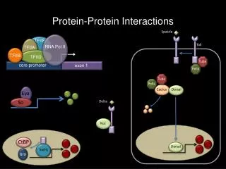
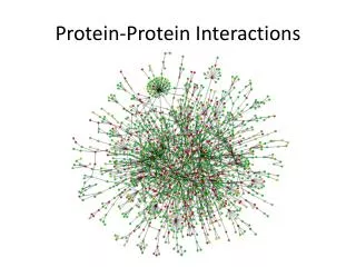
Protein-Protein Interactions. Protein Interactions. A Protein may interact with: Other proteins Nucleic Acids Small molecules. Protein-Protein Interactions: The “ Interactome ”. Experimental methods: Mass Spec, yeast 2-hybrid system, microarrays,… Computational techniques:

E N D
Protein Interactions • A Protein may interact with: • Other proteins • Nucleic Acids • Small molecules
Protein-Protein Interactions: The “Interactome” Experimental methods: Mass Spec, yeast 2-hybrid system, microarrays,… Computational techniques: phylogenic profiles, sequence analysis,… 2 challenges: - find which proteins interact (the partners) - find which residues participate in the interactions
Experimental technique: co-expression Microarray: study the expression of genes as a a function of time, or following treatment with a drug, … Co-expression of genes are usually a sign that the two proteins interact. Gene A Gene B Expression level Time or treatment
Transcription factor Yeast 2-hybrid system Binding Domain Activation Domain Activation Domain Binding Domain
Transcription factor Yeast 2-hybrid system Binding Domain Activation Domain Activation Domain Binding Domain Prot2 Prot1 Activation Domain Binding Domain
Transcription factor Yeast 2-hybrid system Binding Domain Activation Domain Activation Domain Binding Domain Prot2 Prot1 Activation Domain Binding Domain If Prot1 and Prot2 interact: Prot2 Prot1 mRNA Activation Domain Binding Domain Promoter Region Reporter Gene
Yeast 2-hybrid system • In words: • A transcription factor is split into 2 domains • 2 hybrid proteins are designed, each containing one of the two proteins • that are tested • If the two proteins interact, the two domains from the transcription • factor will interact, causing expression of a (detectable) reporter gene • The reporter can be: • - essential, in which case the yeast colony dies if the 2 proteins • do not interact • - reversely, the reporter gene can be attached to a green • fluorescent protein • Unfortunately, the rate of false positive is high (estimated > 45%)
Protein Interactions • Databases of experimental protein interaction data • MIPS: http://mips.helmholtz-muenchen.de/proj/yeast/CYGD/interaction/ • (protein-protein interactions in saccharomyces cerevisae) • InterAct:http://www.ebi.ac.uk/intact/index.html • (protein interactions from literature curation) • DIP:http://dip.doe-mbi.ucla.edu/
Predicting Protein-Protein Interactions • Genome-based approach • (1) Proximity of genes on chromosome • Genes that appear near each other on a chromosome are often expressed • together. • They may interact (need confirmation from biology, or annotation) • Example: operons Gene 3 Gene 2 Gene 1
Predicting Protein-Protein Interactions • Genome-based approach • (2) Homology • If A and B interact and C is homologous to A and D is homologous to B • Then do C and D interact? • They may, if • C&D are from the same species (unless host-pathogen interaction) • The binding surface is conserved • The binding residues are conserved
Predicting Protein-Protein Interactions • Genome-based approach • (2) Gene fusion (Rosetta Stone Protein) (Marcotte and Marcotte, 2002)
Predicting Protein-Protein Interactions • Genome-based approach • (2) Gene fusion: significance n: number of A homologues m: number of B homologues k: number of observed fusion N: size of the database p: probability of fusion Hypergeometric distribution: (Marcotte and Marcotte, 2002)
Predicting Protein-Protein Interactions • Genome-based approach • (2) Phylogenetic profiles (Pellegrini et al, PNAS, 1999)
A web portal to Protein-Protein interactions http://string.embl.de
PPI: example: synthesis of tryptophan neighborhood Gene fusion
PPI: example: synthesis of tryptophan Co-expression
Graph Theory Vertex (node) Cycle Edge -5 Directed Edge (Arc) Weighted Edge 10 7 Molecular interaction networks are mapped as graphs
Useful Operation on Graphs • A graph can be treated as a set of vertices and edges; we can then compute intersection, difference, union… • What is the intersection of my interaction set with all known published interactions? • Filtering • Find all protein interactions where at least one partner is localized in the nucleus • Overall statistics • Find the average number of interactions for cell cycle proteins
Predicting protein interactions from networks (Hogue, Toronto, 2004)
Summary • To understand the function of a protein, we need to find its interacting partners • Experimental methods for protein-protein interactions: Mass spec, 2-hybrid yeast system, structural study • Predicting protein-protein interactions: sequence analysis (neighborhood, gene fusion, co-occurrence), text mining,… • Graph theory to mine protein interaction networks
Enzyme – substrate binding: 2 models Substrate (ligand) Enzyme (receptor) + Lock and Key
Enzyme – substrate binding: 2 models Substrate (ligand) Enzyme (receptor) + Substrate (ligand) Enzyme (receptor) + Lock and Key Induced Fit
One receptor, several ligands… The enzyme (receptor) may bind several ligands in different places: • If the protein binds to several ligands, and the affinity for binding ligands 2,3,… changes after the first ligand is bound, the binding is said to be cooperative: • - Positive cooperativity: the affinity increases • - Negative cooperativity: the affinity decreases • If there is no change, the binding is said to be non cooperative Ligand Receptor Co-factors
Co-factors may induce the fit: allostery Ligand Receptor Ligand binds Co-factors bind Co-factors induce conformational Change: allostery
Predicting binding • Computationally, Lock and Key is the simplest case to predict: • Little or no flexibility need be modeled • 6 degrees of freedom (DOF) • Induced fit is much more difficult • >> 6 degrees of freedom (3 rotations, 3 translations) • Algorithms may need to model the movements of • Side chains and backbone of the receptor • Ligands
“Docking” scenarios “Historical” techniques: Lock and Key Rigid Receptor, Rigid Ligand Rigid Receptor, Flexible Ligand FlexibleReceptor, Rigid Ligand FlexibleReceptor, FlexibleLigand Increasing difficulty Current Research area Hopefully soon…
What is docking? Docking is finding the binding geometry of two interacting molecules with known structures The two molecules (“Receptor” and “Ligand”) can be: - two proteins - a protein and a drug - a nucleic acid and a drug Two types of docking: - local docking: the binding site in the receptor is known, and docking refers to finding the position of the ligand in that binding site - global docking: the binding site is unknown. The search for the binding site and the position of the ligand in the binding site can then be performed sequentially or simulaneously
What is docking? Some more definitions: Two types of docking: - rigid docking: both the receptor and ligand are kept rigid. DOF = 6 (3 position + 3 orientation) - flexible docking: flexibility is allowed for the receptor, or the ligand, or both DOF = 6 + Nfree (3 position + 3 orientation + Nfree bonds)
What is docking? Two types of docking: - bound docking: the goal is to reproduce a known complex, where the starting structures for the receptor and ligand are taken from the structure of the complex (testing docking method) - unbound docking: the structures of the receptor and ligand are taken from data on the unbound molecules (actual docking)
Docking Scoring Criteria • Geometric match: • Prevent overlap between atoms of the receptor and ligand • Maximum shape compatibility • Large surface burial • No large cavity at interface • Energetic Match (Force-field + Statistical potential) • Good hydrogen bonding • Good charge complementarity • Polar/polar contacts favored, polar / non polar contacts disfavoured • Low “free energy”
Docking Search Strategies • Full search • Grid approaches (FFT…) • Directed search • Spherical harmonics surface triangle • Geometric hashing • Pseudo Random • Simulated annealing / Monte Carlo • Genetic algorithms
R L Global Rigid Docking: a FFT approach 1. Representation: Receptor: Assign value to each cell: Exterior: a(i,j) = 0 Surface: a(i,j) = +1 Interior: a(i,j) = -15 R Ligand: Exterior: b(i,j) = 0 Surface: b(i,j) = +1 Interior: b(i,j) = -15 L
R R R L L L Global Rigid Docking: a FFT approach 2. Scoring: Translation Y Translation X where b’ is the grid for the ligand after rotation and translation
Global Rigid Docking: a FFT approach 2. Scoring: Test all possible positions of ligand on receptor: - Test all rotations of ligand - For each rotation, test all translations of ligand grid over receptor grid Score(i,j) = Receptor(i,j)*Ligand(i,j) Rotation R; Translation: T = Tx + Ty + Tz: For each R, this requires N6 operations… But, for a given rotation, this is a correlation product, that can be computed in Fourier Space!
R L Global Rigid Docking: a FFT approach Fourier transform R Discretize A=DFT(a) C=A*B S=iDFT(C) Fourier transform Rotation B=DFT(b) L Discretize Computing cost: N3log(N3)!
DARWIN: An Example of Flexible Docking Program DARWIN uses a force field (CHARMM) for scoring, and a genetic algorithm for searching Genetic algorithm: - Every “solution” is represented by a binary string. -3 genes describe the position (with 0.5 Å resolution) - 3 genes describe the orientation (11.25° resolution) - Each flexible bond is described by one parameter (60° resolution) - The population size is 100-1000 and the number of generation is 10% the population size - The basic operations are: - mutation (P = 0.2) - recombination with one cut (P = 0.4) - recombination with two cuts (P=0.4) - the “death rate” is 5% and the survival rate is 10-30% Taylor, J.S. and Burnett, R.M. (2000). DARWIN: A program for docking flexible molecules. Proteins 41, 173-191
DARWIN: An Example of Flexible Docking Program Taylor, J.S. and Burnett, R.M. (2000). DARWIN: A program for docking flexible molecules. Proteins 41, 173-191
DARWIN: An Example of Flexible Docking Program A test case: binding of Mannopyranoside in Concanavalin A (ConA) Taylor, J.S. and Burnett, R.M. (2000). DARWIN: A program for docking flexible molecules. Proteins 41, 173-191
DARWIN: An Example of Flexible Docking Program No water in docking experiment With water in docking experiment Taylor, J.S. and Burnett, R.M. (2000). DARWIN: A program for docking flexible molecules. Proteins 41, 173-191