Download
1 / 18
180 likes | 280 Views
Probabilistic forecasts of precipitation in terms of quantiles. John Bjørnar Bremnes. Example of quantile forecasts. Methods. Quantile regression: estimate of the -th quantile by where r i observations x i predictors (NWP model output) α i regression parameters

E N D
Probabilistic forecasts of precipitation in terms of quantiles John Bjørnar Bremnes
Methods Quantile regression: estimate of the -th quantile by where ri observations xi predictors (NWP model output) αi regression parameters NOTE: minimization must be repeated for each
Local quantile regression: estimate of the -th quantile at predictor value x by where w() weight function, defined such that weather situations similar to x are given largest weight and, hence, greatest impact on the fit λsmoothing parameter. Fraction of data to be used NOTE: minimization must be repeated for each x (and )
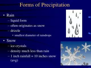
Problem: Precipitation is a discrete/continuous variable Solution: Estimation in two steps • probability of precipitation (discrete) Discriminant analysis, logistic regression (GLM), probit regression (GLM), neural networks, classification trees, … • precip. amounts given occurrence of precip. (continuous) (Local) quantile regression using data with observed precipitation only
Forecasting quantiles Assume the p-th quantile, qp, is of interest • Estimate probability of precipitation, π, at step (i) • Decide which quantile at step (ii) to estimate? • At step (ii) estimate this quantile
Example: • Assume the 5, 25, 50, 75, and 95 percentiles are wanted • probability of precipitation estimated to 0.65 only the 50, 75, and 95 percentiles must be estimated • At step (ii): estimate the 23.1, 61.5, and 92.3 conditional percentiles
Software for quantile regression • Koenker & D’Orey J. R. Statist. Soc., Ser. C, 1987, 36, 383-393 J. R. Statist. Soc., Ser. C, 1993, 43, 410-414http://lib.stat.cmu.edu/apstat/229 (Fortran 77) • R: package “quantreg” (Koenker) http://cran.r-project.org/
Examples: Daily precipitation Location: Brekke i Sogn (north of Bergen, Norway) Data: ECMWF (12+66 UTC) and daily observations (525 days) Experiments EC output from high-resolution model RR, MSLP, RH925-500, RH925-700, Q925-500, Q925-700, DZ925-500, DZ925-700 W, S, F, Vo (basic variables in a Lamb classification algorithm) EPS ALL methods applied to each member, then averaging RR EPS STATS statistics of ensemble as predictors MIN, 5, 25, 50, 75, 95 percentiles, MAX, probability of more than 0.1, 1, 5 mm/day
Selection of predictors/smoothing • Cross-validation (5 parts) Selection based on quality of forecasts • Separately for PoP and amounts given precipitation Verification measures • Probability of precipitation • Brier scores and reliability diagrams • Amounts (conditional quantiles) • Reliability: chi-square test • Sharpness: distribution of prediction intervals (50% and 90%)
EC PoP (probit regression) Log(RR+0.1), W, log(RR+0.1)*W, RH925-500*Vo Amounts (local quantile regression) RR, W, and S Smoothing: 0.7 EPS ALL PoP (probit regression) Log(RR+0.1) Amounts (quantile regression) RR and RR2 EPS STATS PoP (probit regression) Log(MIN+0.1), log(MEDIAN+0.1), log(MAX+0.1) Amounts (local quantile regression) 25 and 75 percentiles of ensemble Smoothing: 0.6
Evaluation and comparison of final forecasts • New cross-validation • Verification as for selecting predictors, but • Quantiles are not conditioned on occurrence of precipitation • Reliability tests (confidence intervals) separately for each quantile • Only cases where quantiles exist are used
Reliability diagrams for probability of precipitation forecasts
Summary of experiments • Raw EPS not reliable (as point forecast) • Best reliable forecasts obtained by using output from the high-resolution model • Forecasts based on ensembles would improve for longer lead times and more variables available • Applying methods to each ensemble member and then averaging, not recommended
Why use quantile regression ? • Produces well-calibrated forecasts • No strong assumptions needed • Any information can be included as predictors • Dealing with ensembles easier • Quantile forecasts ideal for graphical presentations in time
Future work and possibilities • Verification scores for quantile forecasts • Automatic and efficient predictor selection • Local quantile regression • Different predictors for different quantiles • Weighting • Smoothing dependent on quantile • Use of ensembles • Properties of quantile forecasts for extreme events • how to “control” extrapolations • Quantile forecasts for other variables, e.g. wind speed and temperature