Download
1 / 31
310 likes | 421 Views
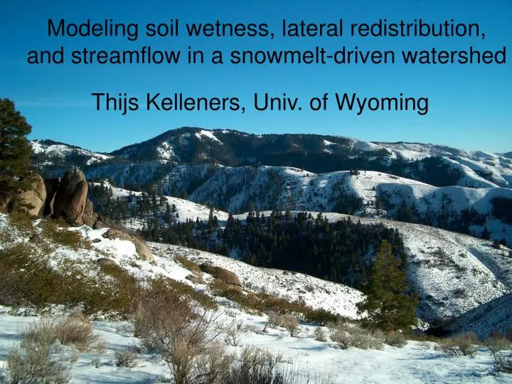
Modeling soil wetness, lateral redistribution, and streamflow in a snowmelt-driven watershed. Thijs Kelleners, Univ. of Wyoming. Water in the Western US. Snowmelt from mountainous areas is an important source of water Rapid snowmelt in the spring may lead to flooding

E N D
Modeling soil wetness, lateral redistribution, and streamflow in a snowmelt-driven watershed Thijs Kelleners, Univ. of Wyoming
Water in the Western US • Snowmelt from mountainous areas is an important source of water • Rapid snowmelt in the spring may lead to flooding • Many interacting factors make it difficult to anticipate the consequences of land management decisions (e.g. grazing, logging, fire) • Effect of climate change on the quantity and timing of runoff
Tools in watershed hydrology • Measure streamflow • Develop rainfall-runoff relationships • Describe the physical processes involved in generating runoff with a computer model • Combine streamflow & point data to test different modeling concepts • Use remotely sensed data to cover large areas • Combine weather/climate predictions with hydrologic models to predict into the future
Physical processes • Net incoming radiation is a function of slope, aspect, and elevation • Vegetation and snowpack modify the surface water & energy fluxes • Surface runoff • Subsurface water flow & heat transport
The energy of water Energy/Volume (Pa=kg/m.s2) Energy/Weight (m) kinetic energy gravitational energy pressure energy osmotic energy z h Hydraulic head (H) = pressure head (h) + gravitational head (z) Darcy equation for flow through porous media:
Modeling water flow (1) St. Venant equations for shallow water flow (potential & kinetic energy) Pro: physically realistic Con: numerical solution difficult Con: surface ponding layer may not be continuous (2a) 3-D Richards’ equation: Pro: physically realistic Con: computationally intensive (2b) 1-D vertical Richards’ equation & 2-D horizontal Boussinesq equation: ; Pro: computationally efficient Con: neglect of lateral unsaturated flow in case of sloping terrain Con: perched water may not be laterally continuous
Simplified approach -Surface runoff: modified Manning’s equation (only the effects of gravity and friction on overland flow are considered): (discharge per unit width) -Lateral subsurface flow: Beven’s approximation for steep slopes (hydraulic gradient is approximately equal to the land surface slope): (discharge per unit width) -Surface ponding: Mass balance equation: (vertical water flux q in m/s) -Soil water flow: 1-D vertical Richards’ equation (using matric flux potential instead of pressure head h; solved through a non-iterative linearization approach) with
Analytical soil hydraulic property functions Sandy loam soil: Air entry pressure head = -0.1466 m Pore-size distribution index = 0.378 Porosity = 0.4 Saturated soil hydraulic conductivity = 0.5077 m/d
Non-iterative solution to 1-D vert. Richards’ eq. 1. For each soil layer we have a mass balance equation: 2. The soil water flux at a fraction through the time step is estimated as: 3. The soil water flux at the beginning of the time step is: 4. The derivatives are: ; 5. The resulting tridiagonal system of eqs. is solved for using Thomas’ algorithm
Vertical soil heat transport -Heat transport is a function of conduction, convection, and sinks/sources: -The soil volumetric heat capacity Cs and the soil thermal conductivity s are not affected by temperature which makes the equation linear -The heat transport equation results in a tridiagonal system of equations that can be solved for soil temperature T using Thomas’ algorithm without iteration
Resulting distributed model • Iterative canopy energy balance ->Tc • Iterative surface energy balance ->Ts • Overland flow • Sub-surface lateral flow • Vertical soil water flow • Vertical soil heat transport • Ponding at the outlet is removed and considered streamflow
Model application for Dry Creek, Boise, ID watershed is divided into 141 10 by 10 m cells movie: relative soil saturation during 18 days in the fall
Model calibration • 1-year period (25-aug-2000 to 24-aug-2001) • Bottom boundary condition: deep percolation into the bedrock is a function of the perched watertable height: qdp=f(H)
Soil water content at the snow sensor location Calculated Measured
Profile-average soil water content at the snow sensor location
Soil temperature at the snow sensor location Calculated Measured
Profile average soil temperature at the snow sensor location
Streamflow at the weir location spring melt period entire period
Summary of results • Snow depth and soil temperature are accurate, indicating that the surface energy balance is correct • Soil water content is overestimated during and after the snow melt period • Streamflow from the watershed is overestimated
Alternative bottom boundary condition • Soil-bedrock interface is generally not smooth • Assumption: top of bedrock behaves as a porous medium • Bottom boundary condition: unit gradient assumption, qdp=K()
Calculated soil water content at the snow sensor location q=K() qdp=f(H)
Profile-average soil water content at the snow sensor location q=K() qdp=f(H)
Streamflow at the weir location q=K() qdp=f(H)
Summary of results • qdp=K() bottom boundary condition results in an underestimation of the soil water content during the melt period • Deep percolation into the bedrock is overestimated will streamflow is underestimated