Download
1 / 40
400 likes | 521 Views
Queen’s University, Kingston April 3 rd 2009. Mapping the intergalactic medium in emission at low and high redshift. Serena Bertone (UC Santa Cruz) Joop Schaye (Leiden Observatory) & the OWLS Team. Outline. Introduction:

E N D
Queen’s University, Kingston April 3rd 2009 Mapping the intergalactic medium in emissionat low and high redshift Serena Bertone (UC Santa Cruz) JoopSchaye (Leiden Observatory) & the OWLS Team
Outline • Introduction: • the intergalactic medium: warm, warm-hot, hot… what is it? • how do we detect it? • New simulations: OWLS • Results: • X-ray & UV emission at z<1 • rest-frame UV emission at z>2 • what gas does emission trace? • dependence on physics
Intergalactic medium: Why do we care? Dark matter: 25% Metals: 0.03% > 90% of the baryonic mass is in diffuse gas (Persic & Salucci 1992, Fukugita et al 1998, Cen & Ostriker 1999) unbiased info on matter power spectrum on largest scales reservoir of fuel for star and galaxy formation IGM metallicityconstrains the cosmic SF history interplay IGM-feedback puts constraints on galaxy formation models Neutrinos: 0.3% Stars: 0.5% Free H & He: 4% Dark energy: 70%
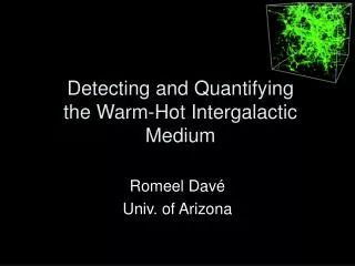
Springel 2003 z=6 z=2 z=0 IGM evolution 100 Mpc cosmictime
Gas temperature distribution T<105 K 105 K <T<107 K T>107 K z=0 Cen & Ostriker 1999 etc Warm-hot gas: WHIM mildly overdense collisionallyionised shock heated by gravitational shocks Hot gas: dense metal enriched haloes of galaxies and clusters Warm gas: diffused photo-ionised traced by Lyα forest
IGM mass and metals The bulk of the metal mass does not trace the bulk of the IGM mass z=0.25 most metal mass most mass Bertone et al. 2009a
Mass and metal fractions evolution IGM mass - Dave’ et al. 2001 Average IGM temperature increases with time Most metals locked in stars at z=0 Average metal temperature increases with time Metal mass - Wiersma et al 2009b halo gas diffuse IGM WHIM ICM
how can we detect the igm? Absorption z<1: UV Tripp et al 2007 Lehner et al 2007 Danforth & Shull 2005 z>1.5: optical Kim et al 2001 Simcoe et al 2006 ✔ ✔? z<1 Nicastro et al 2005 Rasmussen et al 2007 Buote et al 2009 ✔ T<106 K Rest-frame UV lines Lyα, OVI, CIV… T>106 K Soft X-rays metal lines OVII, OVIII, FeXVII ✗ ✗ z<1: UV Furlanetto et al 2004 Bertone et al 2009a z>1.5: optical Weidinger et al 2004 Bertone et al 2009b z<1 Fang et al 2005 Bertone et al 2009a ✔✗ Emission
Owls • OverWhelmingly Large Simulations • The OWLS Team: • JoopSchaye(PI), Claudio DallaVecchia, Rob Wiersma, • Craig Booth, Marcel Haas (Leiden) • Volker Springel (MPA Garching) • Luca Tornatore (Trieste) • Tom Theuns (Durham) • + the Virgo Consortium • Many thanks to the LOFAR and SARA supercomputing facilities
Owls • cosmological hydrodynamical simulations: Gadget 3 • many runs with varying physical prescriptions/numerics • run on LOFAR IBM Bluegene/L • WMAP 3 cosmology • largest runs: 2x5123 particles • two main sets: L=25 Mpc/hand L=100 Mpc/hboxes • evolution from z>100 to z=2 or z=0
New physics in Owls • New star formation (Schaye & DallaVecchia 2008): • Kennicutt-Schmidt SF law implemented without free parameters • New wind model (DallaVecchia & Schaye 2008): • winds local to the SF event • hydrodynamically coupled • Added chemodynamics(Wiersma et al. 2009): • 11 elements followed explicitly (H, He, C, N, O, Ne, Si, Mg, S, Ca, Fe) • Chabrier IMF • SN Ia & AGB feedback • New cooling module (Wiersma, Schaye & Smith 2009): • cooling rates calculated element-by-element from 2D CLOUDY tables • photo-ionisation by evolving UV background included
Physics variations in OWLS • Cosmology: WMAP1 vs WMAP3 vs WMAP5 • Reionisation & Helium reionisation • Gas cooling: primordial abundances vs metal dependent • Star formation: • top heavy IMF in bursts • isothermal & adiabatic EoS • Schmidt law normalisation • Metallicity-dependent SF thresholds • Feedback: • no feedback • feedback intensity: mass loading, initial velocity… • feedback implementation (Springel & Hernquist; Oppenheimer & Dave’) • AGN feedback • Chemodynamics: • ChabriervsSalpeter IMF • SN Ia enrichment • AGB mass transfer
Gas cooling rates collisional ionisation eq. photoionisation eq. density dependent Wiersma, Schaye & Smith 2008 Photo-ionisationby UV BK + collisionalionisation equilibrium Cooling rates calculated element by element for 11 species: takes into account changes in the relative abundances
Gas emissivity z=0.25 UV lines X-ray lines • 11 elements – comparable to cooling rates • Collisionalionisation+ photo-ionisationby UV BKimportant at low density • UV lines stronger than X-ray ones Density Bertone et al 2009a
Emission at low redshift: X-rays 100 Mpc/h boxes 20 Mpc/h thick slices 15” angular resolution 12 emission lines Bertone et al 2009a
X-ray lines O VIII strongest line lines from lower ionisation states and whose emissivity peaks at lower temperatures trace moderately dense IGM: C V, C VI, N VII, O VII, O VIII and Ne IX lines from higher ionisation states trace denser, hotter gas: C VI, O VIII, Ne X, Mg XII, Si XIII, S XV and Fe XVII Fe XVII emission has different spatial distribution than other elements: later enrichment by SN Ia Bertone et al 2009a
What gas produces x-ray emission? emission-weighted particle distributions X-ray emission traces warm-hot, moderately dense gas, not the bulk of the IGM mass and metals. Bertone et al 2009a
Emission at low redshift: UV UV emission is a good tracer of galaxies and of mildly dense IGM, but not of IGM in very dense environments Bertone et al 2009a
UV lines C IV strongest line: traces gas in proximity of galaxies different spatial distribution: O VI and Ne VIII trace more diffuse gas than C IV no emission from the hottest gas in groups
What gas produces UV emission? emission-weighted particle distributions O VI and Ne VIII trace WHIM gas C IV traces more metal-rich, cooler gas Bertone et al 2009a
Summary:Dependencies on gas properties Median density, temperature and metallicity of gas particles vs. particle emission • Correlation of emission with density and metallicity: highest emission from densest and most metal enriched particles • Median temperature of highest emission corresponds to peak temperature of emissivity curve – as seen in T-nHI diagrams Bertone et al 2009a
Impact of physics: x-rays What happens when changing the physical model? • no feedback: no metal transport localised emission • primordial cooling rates: longer cooling times stronger emission at high density (≈100 times) • momentum driven winds: metals more spread in IGM weaker emission (≈100 times) • AGN feedback: weaker emission in dense regions Bertone et al 2009a
Impact of physics: UV • no feedback: emission localised in galaxies • primordial cooling rates: stronger emission at high density • AGN feedback: weaker emission • changes in wind parameters: small effect Bertone et al 2009a
Emission at high redshift:rest-frame UV lines emission at 2<z<5 25 Mpc/h simulations 2” angular resolution Bertone et al 2009b
IGM emission at z>1.5 • At z>1.5 rest-frame UV lines are redshifted in to the optical band • A number of upcoming optical instrument might detect IGM emission lines at 1.5<z<5: • Cosmic Web Imager on Palomar (CWI, Rahman et al 2006) this year! • Keck Cosmic Web Imager (KCWI) • Antarctic Cosmic Web Imager (ACWI, Moore et al 2008) • MUSE on VLT (Bacon et al 2009) • IFUs with large fields of view & high spatial resolution • Great chance to observe the 3-D structure of the IGM for the first time!
Emission PDFs Lower ionisation states: single lines shorter wavelengths C III up to 10x stronger than C IV Higher ionisation states: doublets – easy to identify weaker than lower ion. states
What gas produces UV emission? emission-weighted particle distributions C and Si lines trace colder, more metal enriched gas than O, N and Ne lines Most emission comes from dense gas more metal enriched More highly ionised lines trace warmer gas (e.g. C IV vs C III)
What can we observe with cwi? CWI: flux limit: 100 photon/s/cm2/sr angular resolution: 2” Everything in red and white might be detectable central regions of groups and galactic haloes z=2
summary • Dense cool gas in the haloes of galaxies is traced by: • UV lines: C IV, Si IV • Low density WHIM gas in filaments is traced by: • UV lines: O VI, Ne VIII • soft X-ray lines from hydrogen-like atoms: C V, O VII, Ne IX • soft X-ray lines from elements with low atomic numbers: OVIII • Dense hot gas in clusters and groups is traced by: • soft X-ray lines from fully ionised atoms: C VI, OVIII • soft X-ray lines from elements with high atomic numbers: Mg XII, Fe XVII • Detection of WHIM emission by future telescopes: • challenging in low density regions • very likely in groups and cluster outskirts • CWI very likely to detect metal line emission at high z for the first time
Convergence tests Angular resolution: needed for detecting the spatial distribution of the emitting gas Number of particles: need high resolution for physical processes (star formation, feedback, cooling etc) to converge
Emission per unit volume Most energy emitted by lower ionisation lines: C III, O IV, O V O VI strongest line at higher ionisation Lot of energy emitted by Si lines, despite low emissivity Ne and N emission per unit volume very weak Bertone et al 2009b
Emission vs density • strongest X-ray emission from dense regions • weak emission from the low density, metal poor gas Density cut maps