Download
1 / 1
30 likes | 179 Views
T J Reddish † , D R Tessier † , P Hammond * , A J Alderman * , M R Sullivan † , P A Thorn † and F H Read ‡ † Department of Physics, University of Windsor, Windsor, Canada N9B 3P4 * School of Physics, CAMSP, University of Western Australia, Perth WA 6009, Australia

E N D
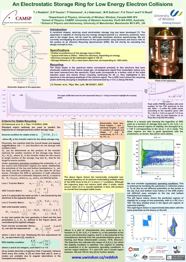
T J Reddish†, D R Tessier†, P Hammond*, A J Alderman*, M R Sullivan†, P A Thorn† and F H Read‡ †Department of Physics, University of Windsor, Windsor, Canada N9B 3P4 *School of Physics, CAMSP, University of Western Australia, Perth WA 6009, Australia ‡ School of Physics and Astronomy, University of Manchester, Manchester M13 9PL, UK Introduction A racetrack shaped, desk-top sized electrostatic storage ring has been developed [1]. The apparatus is capable of storing any low energy charged particle (i.e. electrons, positrons, ions) and in the longer term, will be used for ultra-high resolution electron spectroscopy. We are currently investigating the performance of the spectrometer using electrons and hence refer to the system as an Electron Recycling Spectrometer (ERS). We will shortly be extending this design concept to ions. • Specifications • Orbital circumference of the storage ring is 0.65m. • Typical orbit time is 250ns – 350ns for electrons, depending on energy. • Electrons energies at the interaction region ≤ 150 eV. • Storage lifetimes of ~50 ms have been observed, corresponding to ~200 orbits. Recycling The sharp peaks in the spectrum below correspond primarily to fast electrons that have elastically scattered from helium target gas. (A background signal from metastable helium ions has been removed form the spectrum.) Each peak corresponds to a further orbit of the initial injection pulse and clearly shows recycling continuing for 48 s. Also highlighted in this spectrum is the decaying amplitude of the electron signal. The (x 200) insert shows the recycling peaks uniformly decaying in amplitude and characterized by a 13.6 s decay life-time. An Electrostatic Storage Ring for Low Energy Electron Collisions [1] Tessier et al., Phys. Rev. Lett., 99 253201, 2007. Schematic diagram of the apparatus. Photo of the apparatus. 3·106 Peak width (FWHM) variation with orbit number for the TOF spectrum to the left. After ~ 5 orbits the width varies according to the equation given with W0 = 45.31 ( 0.01) ns and T = 0.74 ns ( 0.01), See [1] and Pedersen et al, Phys Rev A 65 042704 (2002). 2.5·106 x 20 x 200 The upper (x200) data insert has the exponential decay (τ = 13.6ms) removed to highlight the recycling peaks. 2·106 1.5·106 Criteria For Stable Recycling Below is a mosaic plot showing the logarithm of ERS yield as a function of storage time and V2 for V3/V1 = 2. There are several regions of stability, the strongest at V2 = 130 V corresponding to the (H,m) = (2,1) mode. The other regions are also in good agreement with the predictions, as shown. See [2] for more details. Electrostatic thick lens. Focal lengths: f1 and f2; mid-focal lengths: F1 and F2; position of target and image: P and Q, respectively.K1 = P – F1 ; K2 = Q – F2. 1·106 [2] Hammond et al. N. J. Phys. 11 043033, 2009. Standard matrix methods are used to predict the trajectories of charged particles within storage rings. 5·105 0 2 4 6 8 10 12 14 16 18 20 22 24 26 28 30 32 34 36 38 40 42 44 46 48 f1 f2 , Time (ms) General condition for stable orbits is: where Mss is the transfer matrix for the whole storage ring. K1 Physically, this signifies both the overall linear and angularmagnifications are 1, and therefore do not diverge with multiple orbits. Mss can be determined as the product of the transfer matrices for smaller sections of the storage ring. Hence Mss= MstMts, where Mstis the transfer matrix for the source to target section of the storage ring and Mts, that for the target to source section. Under symmetric operating conditions the potentials, V3, of the source and interaction regions are equal. Additionally the potentials of the top and bottom hemispheres, V1, are the same and the potentials, V2, are the same for all four lenses. Therefore the ERS is symmetric in both reflection planes A and B (see schematic diagram) and Mstis equal to Mts. Mst= m2mhm1, where m1,mh, and m2 are defined below. K2 Lens 1 Transfer Matrix: From circular accelerator theory, Mss can also be expressed as: HDA Transfer Matrix: The above figure shows the numerically computed non-paraxial trajectory of an electron undertaking multiple orbits of the ERS close to the H= 2 and m= 1 condition. Although the trajectory does not retrace itself after 2 orbits, which occurs when (2,1) is exactly satisfied, it does still produce an overall time averaged stable beam. Lens 2 Transfer Matrix: We now consider asymmetric operating conditions. This is achieved by breaking the symmetry in reflection plane A. To do this we set different potentials on the lenses in the top (V2t) and bottom (V2b) halves of the ERS and/or set different pass energies to the top and bottom hemispherical analysers. The left figure below shows the predicted regions of stability for a range of lens potentials, with V1t = 9V, V1b = 18V. The blue shaded areas in the figure are regions of expected stability. The right figure below is experimental data taken with the same potentials as the theory on the left. , Lens 2 is physically the same as lens 1, but traversed by the electrons in the opposite direction. Half orbit transfer matrix: In any real system the lens geometry is fixed and the lens parameters f1, f2, K1, K2, defined in the Figure above, are controlled by the applied voltages. Above is a plot of characteristic lens parameters as a function of V2 for V3/V1 = 2 (where V3 is the potential at the source and interaction regions, and V1 is the potential of the hemispheres) derived from the parameterizations given by Harting and Read (Electrostatic Lenses, 1976, Elsevier).The bold blue line indicates the values of K1K2/f1 f2 for which the stability condition is satisfied. Two regions of stability are predicted in V2 for symmetric operating conditions: a narrow region between ~3.1 and 6.8V and a broad region between ~86 and 159.4V. See [2] for further details. ERS stability condition: where θ and Lare real. Employing the two expressions for Mss,as described in [2], results in: where m and H are integers, such that 0 < m< H. (H,m) modes describe a trajectory that, if paraxial, retraces itself every H/m orbits. In [2] we show that odd H, even m modes are unstable due to angular aberrations in the hemispherical analysers. www.uwindsor.ca/reddish